Compare Time-Frequency Content in Signals with Wavelet Coherence
This example shows how to use wavelet coherence and the wavelet cross-spectrum to identify time-localized common oscillatory behavior in two time series. The example also compares the wavelet coherence and cross-spectrum against their Fourier counterparts. You must have Signal Processing Toolbox™ to run the examples using mscohere (Signal Processing Toolbox) and cpsd (Signal Processing Toolbox).
Many applications involve identifying and characterizing common patterns in two time series. In some situations, common behavior in two time series results from one time series driving or influencing the other. In other situations, the common patterns result from some unobserved mechanism influencing both time series.
For jointly stationary time series, the standard techniques for characterizing correlated behavior in time or frequency are cross-correlation, the (Fourier) cross-spectrum, and coherence. However, many time series are nonstationary, meaning that their frequency content changes over time. For these time series, it is important to have a measure of correlation or coherence in the time-frequency plane.
You can use wavelet coherence to detect common time-localized oscillations in nonstationary signals. In situations where it is natural to view one time series as influencing another, you can use the phase of the wavelet cross-spectrum to identify the relative lag between the two time series.
Locate Common Time-Localized Oscillations and Determine Phase Lag
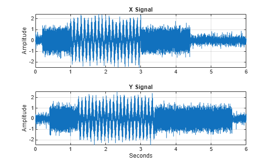
For the first example, use two signals consisting of time-localized oscillations at 10 and 75 Hz. The signals are six seconds in duration and are sampled at 1000 Hz. The 10-Hz oscillation in the two signals overlaps between 1.2 and 3 seconds. The overlap for the 75-Hz oscillation occurs between 0.4 and 4.4 seconds. The 10 and 75-Hz components are delayed 1/4 of a cycle in the Y-signal. This means there is a (90 degree) phase lag between the 10 and 75-Hz components in the two signals. Both signals are corrupted by additive white Gaussian noise.
load wcoherdemosig1
subplot(2,1,1)
plot(t,x1)
title('X Signal')
grid on
ylabel('Amplitude')
subplot(2,1,2)
plot(t,y1)
title('Y Signal')
ylabel('Amplitude')
grid on
xlabel('Seconds')
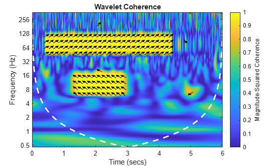
Obtain the wavelet coherence and display the result. Enter the sampling frequency (1000 Hz) to obtain a time-frequency plot of the wavelet coherence. In regions of the time-frequency plane where coherence exceeds 0.5, the phase from the wavelet cross-spectrum is used to indicate the relative lag between coherent components. Phase is indicated by arrows oriented in a particular direction. Note that a 1/4 cycle lag in the Y-signal at a particular frequency is indicated by an arrow pointing vertically.
figure
wcoherence(x1,y1,1000)

The two time-localized regions of coherent oscillatory behavior at 10 and 75 Hz are evident in the plot of the wavelet coherence. The phase relationship is shown by the orientation of the arrows in the regions of high coherence. In this example, you see that the wavelet cross-spectrum captures the (1/4 cycle) phase lag between the two signals at 10 and 75 Hz.
The white dashed line shows the cone of influence where edge effects become significant at different frequencies (scales). Areas of high coherence occurring outside or overlapping the cone of influence should be interpreted with caution.
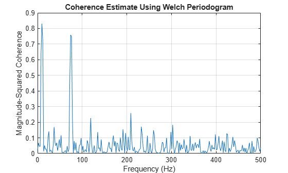
Repeat the same analysis using the Fourier magnitude-squared coherence and cross-spectrum.
figure
mscohere(x1,y1,500,450,[],1000)
[Pxy,F] = cpsd(x1,y1,500,450,[],1000);
Phase = (180/pi)*angle(Pxy);
figure
plot(F,Phase)
title('Cross-Spectrum Phase')
xlabel('Hz')
ylabel('Phase (Degrees)')
grid on
ylim([0 180])
xlim([0 200])
hold on
plot([10 10],[0 180],'r--')
plot([75 75],[0 180],'r--')
plot(F,90*ones(size(F)),'r--')
hold off
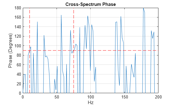
The Fourier magnitude-squared coherence obtained from mscohere (Signal Processing Toolbox) clearly identifies the coherent oscillations at 10 and 75 Hz. In the phase plot of the Fourier cross-spectrum, the vertical red dashed lines mark 10 and 75 Hz while the horizontal line marks an angle of 90 degrees. You see that the phase of the cross-spectrum does a reasonable job of capturing the relative phase lag between the components.
However, the time-dependent nature of the coherent behavior is completely obscured by these techniques. For nonstationary signals, characterizing coherent behavior in the time-frequency plane is much more informative.
The following example repeats the preceding one while changing the phase relationship between the two signals. In this case, the 10-Hz component in the Y-signal is delayed by 3/8 of a cycle ( radians). The 75-Hz component in the Y-signal is delayed by 1/8 of a cycle ( radians). Plot the wavelet coherence and threshold the phase display to only show areas where the coherence exceeds 0.75.
load wcoherdemosig2
wcoherence(x2,y2,1000,'phasedisplaythreshold',0.75)
Phase estimates obtained from the wavelet cross-spectrum capture the relative lag between the two time series at 10 and 75 Hz.
If you prefer to view data in terms of periods rather than frequency, you can use a MATLAB duration object to provide wcoherence with a sample time.
wcoherence(x2,y2,seconds(0.001),'phasedisplaythreshold',0.75)
Note that cone of influence has inverted because the wavelet coherence is now plotted in terms of periods.
Determine Coherent Oscillations and Delay in Climate Data
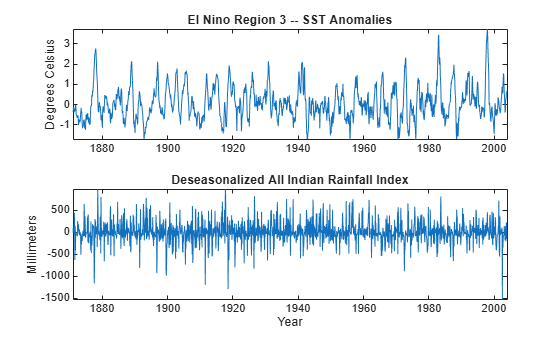
Load and plot the El Nino Region 3 data and deseasonalized All Indian Rainfall Index from 1871 to late 2003. The data are sampled monthly. The Nino 3 time series is a record of monthly sea surface temperature anomalies in degrees Celsius recorded from the equatorial Pacific at longitudes 90 degrees west to 150 degrees west and latitudes 5 degrees north to 5 degrees south. The All Indian Rainfall Index represents average Indian rainfalls in millimeters with seasonal components removed.
load ninoairdata
figure
subplot(2,1,1)
plot(datayear,nino)
title('El Nino Region 3 -- SST Anomalies')
ylabel('Degrees Celsius')
axis tight
subplot(2,1,2)
plot(datayear,air)
axis tight
title('Deseasonalized All Indian Rainfall Index')
ylabel('Millimeters')
xlabel('Year')
Plot the wavelet coherence with phase estimates. For this data, it is more natural to look at oscillations in terms of their periods in years. Enter the sampling interval (period) as a duration object with units of years so that the output periods are in years. Show the relative lag between the two climate time series only where the magnitude-squared coherence exceeds 0.7.
figure
wcoherence(nino,air,years(1/12),'phasedisplaythreshold',0.7)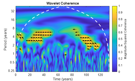
The plot shows time-localized areas of strong coherence occurring in periods that correspond to the typical El Nino cycles of 2 to 7 years. The plot also shows that there is an approximate 3/8-to-1/2 cycle delay between the two time series at those periods. This indicates that periods of sea warming consistent with El Nino recorded off the coast of South America are correlated with rainfall amounts in India approximately 17,000 km away, but that this effect is delayed by approximately 1/2 a cycle (1 to 3.5 years).
Find Coherent Oscillations in Brain Activity
In the previous examples, it was natural to view one time series as influencing the other. In these cases, examining the lead-lag relationship between the data is informative. In other cases, it is more natural to examine the coherence alone.
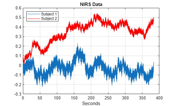
For an example, consider near-infrared spectroscopy (NIRS) data obtained in two human subjects. NIRS measures brain activity by exploiting the different absorption characteristics of oxygenated and deoxygenated hemoglobin. The data is taken from Cui, Bryant, & Reiss [1] and was kindly provided by the authors for this example. The recording site was the superior frontal cortex for both subjects. The data is sampled at 10 Hz. In the experiment, the subjects alternatively cooperated and competed on a task. The period of the task was approximately 7.5 seconds.
load NIRSData
figure
plot(tm,NIRSData(:,1))
hold on
plot(tm,NIRSData(:,2),'r')
legend('Subject 1','Subject 2','Location','NorthWest')
xlabel('Seconds')
title('NIRS Data')
grid on
hold off
Obtain the wavelet coherence as a function of time and frequency. You can use wcoherence to output the wavelet coherence, cross-spectrum, scale-to-frequency, or scale-to-period conversions, as well as the cone of influence. In this example, the helper function helperPlotCoherence packages some useful commands for plotting the outputs of wcoherence.
[wcoh,~,F,coi] = wcoherence(NIRSData(:,1),NIRSData(:,2),10,'numscales',16);
helperPlotCoherence(wcoh,tm,F,coi,'Seconds','Hz')
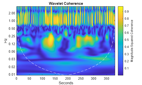
In the plot, you see a region of strong coherence throughout the data collection period around 1 Hz. This results from the cardiac rhythms of the two subjects. Additionally, you see regions of strong coherence around 0.13 Hz. This represents coherent oscillations in the subjects' brains induced by the task. If it is more natural to view the wavelet coherence in terms of periods rather than frequencies, you can input the sampling interval as a duration object. wcoherence provides scale-to-period conversions.
[wcoh,~,P,coi] = wcoherence(NIRSData(:,1),NIRSData(:,2),seconds(0.1),...
    'numscales',16);
helperPlotCoherence(wcoh,tm,seconds(P),seconds(coi),...
    'Time (secs)','Periods (Seconds)')
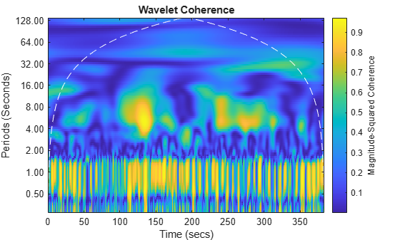
Again, note the coherent oscillations corresponding to the subjects' cardiac activity occurring throughout the recordings with a period of approximately one second. The task-related activity is also apparent with a period of approximately 8 seconds. Consult Cui, Bryant, & Reiss [1] for a more detailed wavelet analysis of this data.
Conclusions
In this example you learned how to use wavelet coherence to look for time-localized coherent oscillatory behavior in two time series. For nonstationary signals, it is often more informative if you have a measure of coherence that provides simultaneous time and frequency (period) information. The relative phase information obtained from the wavelet cross-spectrum can be informative when one time series directly affects oscillations in the other.
Appendix
The following helper function is used in this example.
References
[1] Cui, X., D. M. Bryant, and A. L. Reiss. "NIRS-Based Hyperscanning Reveals Increased Interpersonal Coherence in Superior Frontal Cortex during Cooperation." Neuroimage. Vol. 59, Number 3, 2012, pp. 2430–2437.
[2] Grinsted, A., J. C. Moore, and S. Jevrejeva. "Application of the cross wavelet transform and wavelet coherence to geophysical time series." Nonlinear Processes in Geophysics. Vol. 11, 2004, pp. 561–566. doi:10.5194/npg-11-561-2004.
[3] Maraun, D., J. Kurths, and M. Holschneider. "Nonstationary Gaussian processes in wavelet domain: synthesis, estimation, and significance testing." Physical Review E. Vol. 75, 2007, pp. 016707(1)–016707(14). doi:10.1103/PhysRevE.75.016707.
[4] Torrence, C., and P. Webster. "Interdecadal Changes in the ENSO-Monsoon System." Journal of Climate. Vol. 12, Number 8, 1999, pp. 2679–2690. doi:10.1175/1520-0442(1999)012<2679:ICITEM>2.0.CO;2.