wtmm

Wavelet transform modulus maxima

Syntax

hexp = wtmm(x)

[hexp,tauq] = wtmm(x)

[___] = wtmm(x,MinRegressionScale=scale)

[hexp,tauq,structfunc] = wtmm(___)

[localhexp,wt,wavscales] = wtmm(x,ScalingExponent="local")

wtmm(___,ScalingExponent="local")

[___] = wtmm(___,Name=Value)

Description

hexp = wtmm(x) returns an estimate of the global Hölder exponent, hexp, for x.

[hexp,tauq] = wtmm(x) also returns an estimate of the partition function scaling exponents, tauq.

[___] = wtmm(x,MinRegressionScale=scale) uses only scales greater than or equal to scale to estimate the global Hölder exponent. This syntax can include any of the output arguments used in previous syntaxes.

[hexp,tauq,structfunc] = wtmm(___) also returns the multiresolution structure functions, structfunc, for the global Hölder exponent estimate. This syntax can include any of the input arguments used in previous syntaxes.

[localhexp,wt,wavscales] = wtmm(x,ScalingExponent="local") returns the local Hölder exponent estimates localhexp, the continuous wavelet transform (CWT) of the signal, wt, and the scales wavscales used in the CWT.

wtmm(___,ScalingExponent="local") with no output arguments plots the wavelet maxima lines in the current figure. Estimates of the local Hölder exponents are displayed in a table to the right of the plot.

[___] = wtmm(___,Name=Value) returns the Hölder exponent and other specified outputs with additional options specified by one or more Name=Value arguments.

Examples

Global Hölder Exponent for Brownian Motion

Estimate the global Hölder exponent for Brownian motion. This monofractal signal has a Hölder exponent of approximately 0.5.

rng(100)
x = cumsum(randn(2^15,1));
hexp = wtmm(x)

hexp = 
0.4958

Linearity of Scaling Exponents for Monofractal Signal

Confirm that for a monofractal signal, the scaling exponents are a linear function of the moments. For multifractal signals, the exponents are a nonlinear function of the moments.

Load a signal that contains two time series, each with 8000 samples. Ts1 is a multifractal signal and Ts2 is a monofractal fractional Brownian signal. Obtain the exponents using wtmm.

load RWdata
[hexp1,tauq1] = wtmm(Ts1);
[hexp2,tauq2] = wtmm(Ts2);

Plot the scaling exponents.

expplot = plot(-2:0.1:2,tauq2,"b-o",-2:0.1:2,tauq1,"r-^");
grid on
expplot(1).MarkerFaceColor = "b";
expplot(2).MarkerFaceColor = "r";
legend("Ts2-Monofractal","Ts1-Multifractal",Location="SouthEast")
title("Monofractal vs. Multifractal Scaling Exponents")
xlabel("Qth Moment")
ylabel("Scaling Exponents")

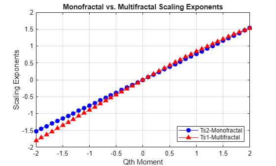
Ts2, which is the monofractal signal, is a linear function. Ts1, the multifractal signal, is not linear.

Structure Function of Wavelet Transform Modulus Maxima

Use the structure function output of wtmm to analyze a Brownian motion signal.

Create fractional Brownian motion with a Hölder exponent of 0.6.

Brn = wfbm(0.6,2^15);
[hexp,tauq,structfunc] = wtmm(Brn);

Compare the calculated Hölder exponent with the theoretical value of 0.6.

hexp

hexp = 
0.6127

Use the data in the structfunc output and the lscov function to perform the regression on the data.

x = ones(length(structfunc.logscales),2);
x(:,2) = structfunc.logscales;
betahat = lscov(x,structfunc.Tq,structfunc.weights);
betahat = betahat(2,:);

Plot and compare the scaling exponents from the tauq output and from the regressed structure function output.

tiledlayout(1,2)
nexttile
plot(-2:.1:2,tauq)
grid on
title("From tauq Output")
xlabel("Qth Moment")
ylabel("Scaling Exponents")
nexttile
plot(-2:.1:2,betahat(1:41))
grid on
title("From structfunc Output")
xlabel("Qth Moment")

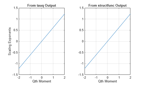
The plots are the same and show a linear relationship between the moments and the exponents. Therefore, the signal is monofractal. The Hölder exponent returned in hexp is the slope of this line.

Local Hölder Exponents for Cusp Signal and Delta Functions

Using a cusp signal and a signal containing delta functions, generate their local Hölder exponents.

Cusp Signal

Load and plot a cusp signal. Note the difference between the two cusps.The cusp signal has Hölder exponents of 0.5 and 0.3 at samples 241 and 800, respectively. The higher Hölder value at sample 241 indicates that the signal at that point is closer to being differentiable than the signal at sample 800, which has a smaller Hölder value.

load cusp
plot(cusp)
grid on
xlabel("Sample")
ylabel("Amplitude")

Obtain the local Hölder exponents and plot the modulus maxima. The WTMM algorithm builds a skeleton of maxima across scales, and the computed exponents and locations differ only slightly from the theoretical values.

wtmm(cusp,ScalingExponent="local")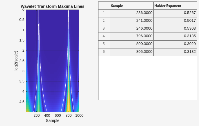

Delta Functions

Create and plot two delta functions.

x = zeros(1e3,1);
x([200 500]) = 1;  
plot(x)
grid on
xlabel("Sample")
ylabel("Amplitude")

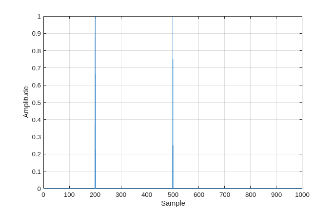
Obtain the local Hölder exponents using the default number of octaves, which in this case is 7. Plot the modulus maxima. A delta function has a Hölder exponent of -1.

wtmm(x,ScalingExponent="local")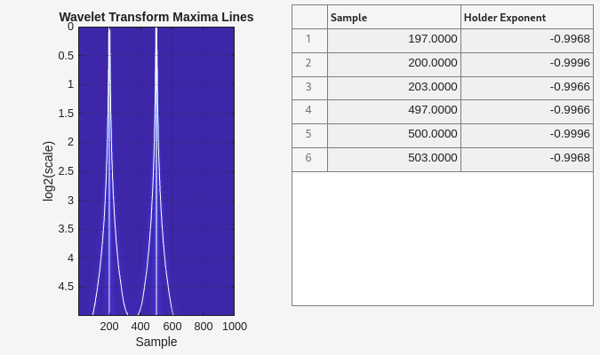

Obtain the local Hölder exponents using 5 octaves and compare the modulus maxima plot to the plot using the default number of octaves.

wtmm(x,ScalingExponent="local",NumOctaves=5)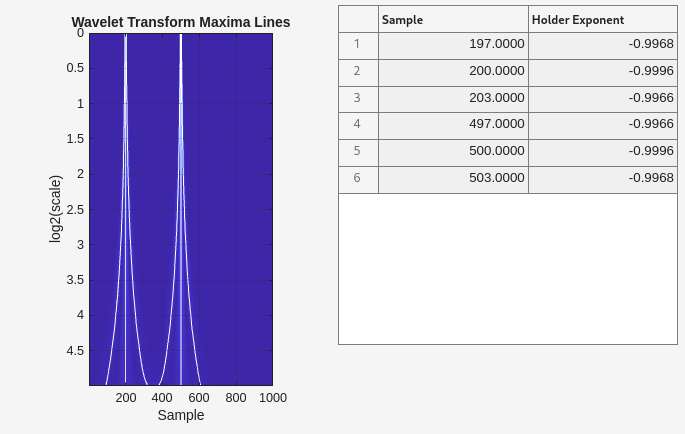

Reducing the number of scales provides more separation in frequency and less overlap between the modulus maxima lines of the delta functions.

Input Arguments

x — Input signal

vector

Input signal, specified as a real-valued vector with a minimum of 128 samples. The wavelet transform modulus maxima technique works best for data with 8000 or more samples.

Data Types: double

Name-Value Arguments

Specify optional pairs of arguments as Name1=Value1,...,NameN=ValueN, where Name is the argument name and Value is the corresponding value. Name-value arguments must appear after other arguments, but the order of the pairs does not matter.

Example: hexp = wtmm(x,ScalingExponent="global",VoicesPerOctave=18) estimates the global Hölder estimate using 18 voices per octave.

Before R2021a, use commas to separate each name and value, and enclose Name in quotes.

Example: hexp = wtmm(x,'ScalingExponent',"global",'VoicesPerOctave',18) estimates the global Hölder estimate using 18 voices per octave.

MinRegressionScale — Minimum scale for regression

4 (default) | scalar greater than or equal to 4

Minimum scale for regression, specified as a scalar greater than or equal to 4. This scale is the smallest scale used by the regression. There must be at least two scales with more than six CWT maxima. MinRegressionScale applies only to global Hölder exponents.

VoicesPerOctave — Number of voices per octave

10 (default) | even integer from 8 to 32

Number of voices per octave, specified as an even integer from 8 to 32. The number of voices per octave and the number of octaves determine the number of scales used in the CWT.

NumOctaves — Number of octaves

minimum of 7 and floor(log2(numel(x)/(8*sigmat))) (default) | integer greater than or equal to 2

Number of octaves, specified as an integer greater than or equal to 2. The number of octaves and the number of voices per octave determine the number of scales used in the CWT. The maximum number of octaves is less than or equal to floor(log2(numel(x)/(8*sigmat))), where sigmat is the standard deviation of the second derivative of the Gaussian wavelet in time. The value of the standard deviation is approximately 2.0861. By default, the number of octaves is the minimum of 7 and floor(log2(numel(x)/(8*sigmat))). If you specify the number of octaves as greater than the maximum allowable number, wtmm uses the maximum supported number of octaves.

ScalingExponent — Type of scaling exponents

"global" (default) | "local"

Type of scaling exponents, specified as one of these:

• "global" — A global Hölder exponent is used for monofractal signals, such as white noise, which are singular everywhere. Global Hölder exponents give a single estimate of degree of these singularities over the whole signal.

• "local" — Local Hölder exponents are useful for signals with cusp singularities.

Output Arguments

hexp — Global Hölder exponent

scalar

Global Hölder exponent, returned as a real-valued scalar. The wtmm function estimates hexp by regressing the mean log of the CWT maxima by scale on the log of the wavelet scales. For the CWT, wtmm uses the 2nd derivative of the Gaussian wavelet.

Hölder exponents are useful for identifying singularities, which are locations where a signal is not differentiable. A global Hölder exponent uses a single value to estimate the degree of differentiability of all of the singularities of a signal. Signals with a global Hölder exponent are monofractal signals. To analyze multifractal signals, use dwtleader.

The wavelet transform modulus maxima method (WTMM) identifies cusp-like singularities in a signal. For more information, see Algorithms

tauq — Scaling exponents

column vector

Scaling exponents, returned as a column vector. The exponents are estimated for the linearly-spaced q-moments of the structure functions from –2 to +2 in 0.1 increments.

structfunc — Multiresolution structure functions

structure array

Multiresolution structure functions for the global Hölder exponent estimates, returned as a structure array. The structure function for data x is defined as

$$S(q,a)=\frac{1}{n_a}{\displaystyle \sum _{k=1}^{n_a}{\left|T_x(a,k)\right|}^q}\simeq a^{\zeta (q)},$$

where a is the scale, q is the moment, T_x is the maxima at each scale, n_a is the number of maxima at each scale, and $$\zeta (q)$$ is the scaling exponent. structfunc is a structure array containing the following fields:

• Tq — Measurements of the input, x, at various scales. Tq is a matrix of multiresolution quantities that depend jointly on time and scale. Scaling phenomena in x imply a power-law relationship between the moments of Tq and the scale. Tq is an Ns-by-44 matrix, where Ns is the number of scales. The first 41 columns of Tq contain the scaling exponent estimates for each of the q-moments from –2 to +2 in 0.1 increments, by scale. The last three columns correspond to the first-order, second-order, and third-order cumulants, respectively, by scale. For a monofractal signal, cumulants greater than the first cumulant are zero.

• weights — Weights used in the regression estimates. The weights correspond to the number of wavelet maxima at each scale. weights is an Ns-by-1 vector.

• logscales — Scales used as predictors in the regression. logscales is an Ns-by-1 vector with the base-2 logarithm of the scales.

localhexp — Local Hölder exponent estimates

array of real values

Local Hölder exponent estimates, returned as an M-by-2 array of real values, where M is the number of maxima. The first column contains the sample of the local singularity, and the second column is the estimated Hölder exponent. If no maxima lines converge to the finest scale in the wavelet transform, then localhexp is an empty array.

The wavelet transform modulus maxima method (WTMM) identifies cusp-like singularities in a signal. For more information, see Algorithms

wt — Continuous wavelet transform

matrix

Continuous wavelet transform of the signal, returned as a matrix of real values. wt is a numel(wavscales)-by-N matrix, where N is the length of the input signal x.

wavscales — Wavelet scales

column vector

Wavelet scales, returned as a column vector of real values. wavscales are the scales used to calculate the CWT.

More About

Modulus Maximum

For the wavelet transform of f, Wf(s,x), the point x₀ and scale s₀ is a modulus maximum if

$$\left|Wf(s_0,x)\right|<\left|Wf(s_0,x_0)\right|,$$

where x is either in the right or left neighborhood of x₀, and

$$\left|Wf(s_0,x)\right|\le \left|Wf(s_0,x_0)\right|,$$

when x belongs to the opposite neighborhood of x₀.

Hölder exponent

Hölder exponents indicate the degree of differentiability for each singularity in a signal. The exponent classifies the singularity strength.

• A Hölder exponent less than or equal to 0 indicates a discontinuity at that location.

• A Hölder exponent greater than or equal to 1 indicate that the signal is differentiable at that location.

• Hölder exponents between 0 and 1 indicate continuous, but not differentiable locations.

Hölder exponents indicate how close the signal at that sample is to being differentiable. Hölder exponents close to 0 indicate signal locations that are less differentiable than locations with exponents closer to 1. The signal is smoother at locations with higher local Hölder exponents.

Algorithms

The WTMM algorithm finds singularities in a signal by determining maxima. The WTMM is intended to be used with large data sets so that enough samples are available to determine maxima accurately.

An overview of the algorithm follows.

1. The algorithm calculates the continuous wavelet transform (CWT) using the second derivative of the Gaussian wavelet with 10 voices per octave. The Ricker wavelet meets this criteria.

2. At the initial scale, the algorithm determines the modulus maxima.

3. The algorithm continues up through finer scales, finding the modulus maxima and checking whether the maxima align between scales. If a maximum converges to the finest scale, it is a true maximum and indicates a singularity at that point.

4. When each singularity is determined, the algorithm estimates its Hölder exponent.

For signals with a few cusp-like singularities and Hölder exponents that have large variation, you set the algorithm to return local Hölder exponents, which provide individual values for each singularity. For signals with numerous Hölder exponents that have relatively small variations, you set the algorithm to return a global Hölder exponent. A global Hölder exponent applies to the whole signal. For signals with many singularities, you can reduce the number of maxima found by limiting the algorithm to start at or regress to a specific minimum or maximum scale, respectively. For detailed information about the WTMM, see [1] and [3].

References

[1] Mallat, S., and W.L. Hwang. “Singularity Detection and Processing with Wavelets.” IEEE Transactions on Information Theory 38, no. 2 (March 1992): 617–43. https://doi.org/10.1109/18.119727.

[2] Wendt, Herwig, and Patrice Abry. “Multifractality Tests Using Bootstrapped Wavelet Leaders.” IEEE Transactions on Signal Processing 55, no. 10 (October 2007): 4811–20. https://doi.org/10.1109/TSP.2007.896269.

[3] Arneodo, Alain, Benjamin Audit, Nicolas Decoster, Jean-Francois Muzy, and Cedric Vaillant. “Wavelet Based Multifractal Formalism: Applications to DNA Sequences, Satellite Images of the Cloud Structure, and Stock Market Data.” In The Science of Disasters, by Armin Bunde, Jürgen Kropp, and Hans Joachim Schellnhuber, 26–102. Berlin, Heidelberg: Springer Berlin Heidelberg, 2002. https://doi.org/10.1007/978-3-642-56257-0_2.

Version History

Introduced in R2016b