Obtain Orthophotos from Central Perspective Images

Step 2 of 4 in Map and Classify Urban Environment Using UAV Camera and Deep Learning

After modeling a UAV flying over the US City Block scene and capturing central perspective images, as described in the Survey Urban Environment Using UAV example, convert the central perspective images into orthographic photos. Real-world cameras, like the ones on UAVs, can capture only perspective images. However, applications of aerial photogrammetry, such as city mapping, require orthographic images.

Background

Aerial photogrammetry involves the creation of accurate maps of the terrain. Maps, having a uniform scale, provide orthographic views of surfaces of interest, which makes accurate terrain measurements possible. You obtain these maps by stitching images of uniform scale together in a process known as homography or image stitching. For more information on this process, see the Create Panorama (Computer Vision Toolbox) example. Images obtained by real-world cameras, however, provide perspective projections of the world. This makes image stitching difficult, because perspective images do not have a uniform scale. For more information on the difference between perspective projection and orthographic projection, see Understanding View Projections. To enable easier image stitching, you must convert perspective images into orthophotos, which have a uniform scale [1]. You can then stitch the orthophotos into an orthomosaic, which is your final map of the terrain of interest. For more information about orthophotos, see the Appendix section.

The primary purpose for converting aerial photographs acquired by UAVs into orthophotos is to obtain the ground plane.

In this example, you obtain orthophotos from central perspective images captured by a UAV. For this conversion, you use these parameters:

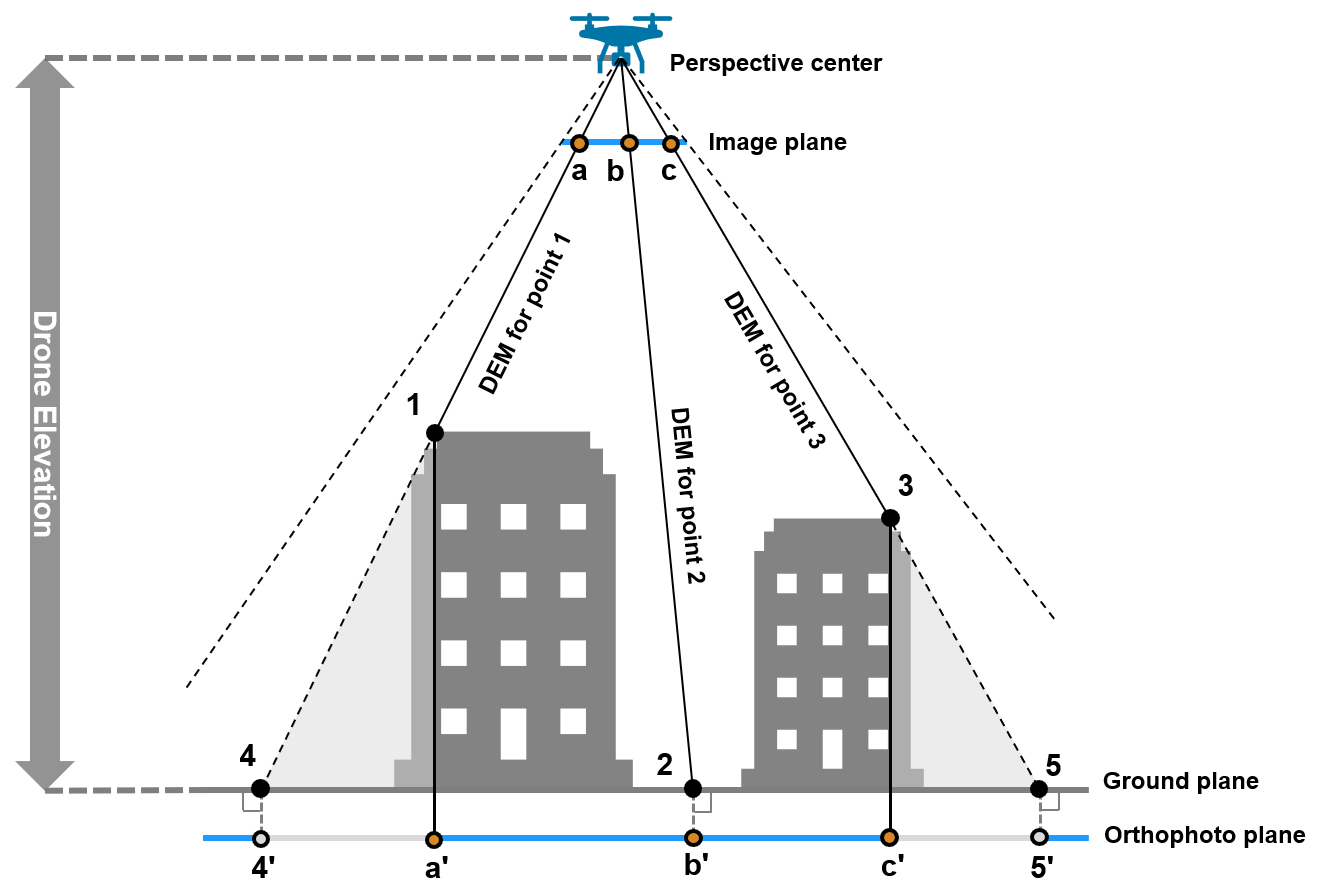
• Digital Elevation Model (DEM) — Also known as the depth map, the digital elevation model is a matrix obtained by a depth sensor on the UAV that provides the distance of the real-world point of each pixel from the perspective center. For point 1, this would be the distance between the perspective center and the yellow point 1 as shown in this diagram of the appendix, and similarly for yellow points 2 and 3.

• Camera Parameters — The intrinsic and extrinsic parameters of the camera. For more information, see Camera Calibration Parameters (Computer Vision Toolbox). This includes the location of the lens with respect to the image plane and the elevation of the UAV as shown in this diagram.

• Meter to Pixel Ratio — The ratio between real-world units, meters, and the pixels of your monitor. Use this ratio to convert meters into pixel units.

Setup

If you have not run the Survey Urban Environment Using UAV example, you can download that data for this example by setting ranPrevEx to false. Otherwise, set ranPrevEx to true.

ranPrevEx = "false";

If ranPrevEx is false, download the required data.

if strcmp(ranPrevEx,"false")
    preAcquiredDataComponent = "uav/data/R2023b";
    preAcquiredDataFilename = "flightData.zip";
    disp("Downloading previously acquired flight data (300 MB)...");
    preAcquiredDataFolder = exampleHelperDownloadData(preAcquiredDataComponent,preAcquiredDataFilename);
end

Downloading previously acquired flight data (300 MB)...

Load Data Acquired by UAV Flight

Load the flightData MAT file, which contains this data, into the workspace:

• image — Image frames acquired by the UAV camera for each time step, returned as an H-by-W-by-3-by-F array.

• depth — Depth map for each image frame acquired by the UAV camera, returned as an H-by-W-by-F array.

• focalLength — The focal length of the UAV camera, in meters. Note that the UAV camera in this example is facing vertically downward.

• meterToPixel — The number of pixels on your screen that constitute 1 meter in the real world. This is also the ratio between your screen and the Simulink space. The value in the downloaded data has been calculated for a screen on which 752 pixels corresponds to 15.6 cm in the real world. If this value does not match your monitor, adjust it accordingly.

• reductionFactor — This value represents the reduction factor for each axis. If the saved orthophoto [H W] size pixels, then the actual size of the orthophoto is [H W]⋅reductionFactor in pixels, and the real-world size of the orthophoto, in meters, is [H W]⋅reductionFactor⋅meterToPixel. This ensures that 1 meter in this final map is equivalent to 1 meter in real life. Because processing matrices with millions of rows and columns is computationally expensive, you use the reduction factor to scale down such matrices.

$\mathit{H}$ and $\mathit{W}$ are the height and width in pixels of the acquired image, respectively. $\mathit{F}$ is the total number of time steps logged and is directly proportional to the flight time.

If indicated that you ran the Survey Urban Environment Using UAV example, a dialog box opens and prompts you to select the path to the flightData.mat file generated by that example.

if strcmp(ranPrevEx,"true")
    [file,path] = uigetfile("flightData.mat","Select flightData.mat file to open",MultiSelect="off");
    load([path file]);
else
    preAcquiredFlightData = fullfile(preAcquiredDataFolder,"flightData.mat");  
    load(preAcquiredFlightData);
end

Convert Perspective Images into Orthophotos

To capture the central perspective images, first obtain the image resolution of the camera.

persImgResX = size(image,1);
persImgResY = size(image,2);

If an orthophotos folder does not already exist in the current working directory, create this folder to store the computed orthophotos.

orthophotoFolderName = "orthophotos";
exampleHelperMakeFolder(orthophotoFolderName);

Obtain the total number of frames, and create an empty cell array to store the orthophotos for computation.

numberOfFrames = size(image,4);
orthophotos = cell(1,numberOfFrames);

Convert each frame into an orthophoto by using the exampleHelperGetOrthoFromPers helper function, and save each orthophoto in the orthophotos folder.

% Show progress bar
f = waitbar(0,"Please wait while orthophoto images are being written ...");

% Convert each frame into an orthophoto
for idx=1:numberOfFrames
    
    % Compute orthophoto for current frame and then save it as an image file
    orthophotos{idx} = exampleHelperGetOrthoFromPers(focalLength,persImgResX,persImgResY,...
        targetUAVElevation,meterToPixel,reductionFactor,...
        image(:,:,:,idx),depth(:,:,idx));
    imwrite(orthophotos{idx}/255,fullfile(orthophotoFolderName,"frame_"+string(idx)+".png"));
    
    % Update the progress bar
    progress = idx/numberOfFrames;
    waitbar(progress,f,sprintf("Creating files for frame [%d/%d] - %.2f%%",idx,numberOfFrames,progress*100));
end
% Close progress bar
close(f);

Visualize Computed Orthophoto

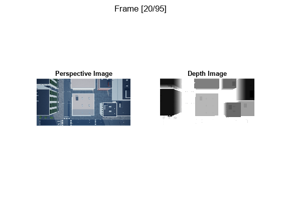
Obtain the perspective image and depth map for frame 20.

sampleIndex = 20;
sampleImage = image(:,:,:,sampleIndex);
sampleDepth = depth(:,:,sampleIndex);

Currently, the depth map is a 2-D matrix of floating point values, such as 53.43, for each pixel. To visualize these values in a [0, 1] color channel scale, you must first normalize them.

Normalize the depth map into the [0, 1] range to visualize it as a monochromatic image.

minDepth = min(sampleDepth,[],"All");
maxDepth = max(sampleDepth,[],"All");
sampleScaledDepth = (sampleDepth-minDepth)/(maxDepth-minDepth);

Visualize the perspective image and its normalized depth map.

subplot(1,2,1)
imshow(sampleImage)
title("Perspective Image")
subplot(1,2,2)
imshow(sampleScaledDepth)
title("Depth Image")
sgtitle(sprintf("Frame [%d/%d]",sampleIndex,numberOfFrames))

Visualize the computed orthophoto for the same frame.

figure
imshow(orthophotos{sampleIndex}/255)
title(sprintf("Orthophoto for Frame [%d/%d]",sampleIndex,numberOfFrames))

Conclusion

This example showed you how to obtain orthophotos from central perspective images and depth sensor information.

In the next step of the Map and Classify Urban Environment Using UAV Camera and Deep Learning workflow, Semantic Segmentation of Orthophotos, you perform semantic segmentation of these orthophotos using a pretrained network.

Appendix

In concept, you can visualize orthophotos from the side like this:

where,

• The camera of the UAV is facing down with a pitch of 0 degrees, acquiring a central perspective image.

• Points $\mathit{a}$, $\mathit{b}$, and $\mathit{c}$ belong to the image plane. The image plane is the central perspective image obtained by the UAV camera.

• Points $1$, $2$, and $3$ correspond to where points $\mathit{a}$, $\mathit{b}$, and $\mathit{c}$ are in the real world, respectively. These points are visible to the UAV, and correspond to the points ${\mathit{a}}^{\prime }$, ${\mathit{b}}^{\prime }$, and ${\mathit{c}}^{\prime }$, respectively, on the orthophoto plane.

• Points $4$ and $5$ are real-world points that are invisible to the UAV. These correspond to points $4^{\prime }$ and $5^{\prime }$, respectively, on the othophoto plane.

• The regions highlighted in grey are also invisible to the UAV due to obstruction caused by the buildings. Note that only a few such representative areas have been highlighted in this diagram. The diagram does not account for all obstructed areas in the image.

The orthophoto plane is also known as the orthophoto or orthomap. The diagram shows how there can be missing areas in an orthophoto as compared to a perspective image for the same scene but an orthophoto is the best approximation of the ground plane from a central perspective image. Ideally you want to obtain the true ground plane, but, the missing areas in the orthophoto demonstrate why you must use multiple views to improve the completeness and accuracy of your map.

References

[1] Lin Y-C, Zhou T, Wang T, Crawford M, Habib A. "New Orthophoto Generation Strategies from UAV and Ground Remote Sensing Platforms for High-Throughput Phenotyping." Remote Sensing. 2021; 13(5):860.

Map and Classify Urban Environment Using UAV Camera and Deep Learning

Next