loss
Evaluate accuracy of learned feature weights on test data
Syntax
Description
err = loss(mdl,Tbl,ResponseVarName)mdl, for the
predictors in table Tbl, and the variable
ResponseVarName in table Tbl. Use this
syntax if mdl was originally trained on a table.
Examples
Load the ionosphere data set, which includes radar signal data. X contains the predictor data, and Y is the response variable, whose values represent either good ("g") or bad ("b") radar signals.
load ionospherePerform neighborhood component analysis (NCA) to identify the important predictors for correctly classifying the radar returns.
mdl = fscnca(X,Y)
mdl =
  FeatureSelectionNCAClassification
          NumObservations: 351
          ModelParameters: [1×1 struct]
                   Lambda: 0.0028
                FitMethod: 'exact'
                   Solver: 'lbfgs'
        GradientTolerance: 1.0000e-06
           IterationLimit: 1000
                PassLimit: 5
      InitialLearningRate: []
                  Verbose: 0
    InitialFeatureWeights: [34×1 double]
           FeatureWeights: [34×1 double]
                  FitInfo: [1×1 struct]
                       Mu: []
                    Sigma: []
                        X: [351×34 double]
                        Y: {351×1 cell}
                        W: [351×1 double]
               ClassNames: {2×1 cell}


  Properties, Methods
mdl is a FeatureSelectionNCAClassification model object that contains the data, fitting information, feature weights and other parameters of the NCA model. Plot the feature weights. The weights of the unimportant features are close to zero.
figure()
plot(mdl.FeatureWeights,"o")
grid on
xlabel("Feature Index")
ylabel("Feature Weight")

Compute the misclassification error of the NCA model.
L = loss(mdl,X,Y)
L =
0.0142
Load the sample data.
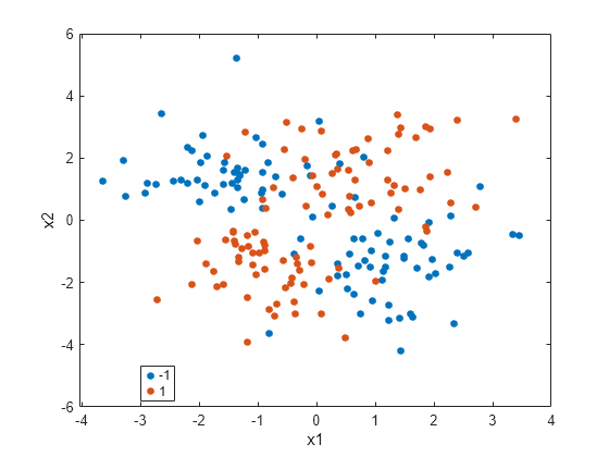
load("twodimclassdata.mat")This data set is simulated using the scheme described in [1]. This is a two-class classification problem in two dimensions. Data from the first class (class –1) are drawn from two bivariate normal distributions or with equal probability, where , , and . Similarly, data from the second class (class 1) are drawn from two bivariate normal distributions or with equal probability, where , , and . The normal distribution parameters used to create this data set result in tighter clusters in data than the data used in [1].
Create a scatter plot of the data grouped by the class.
gscatter(X(:,1),X(:,2),y)
xlabel("x1")
ylabel("x2")
Add 100 irrelevant features to . First generate data from a Normal distribution with a mean of 0 and a variance of 20.
n = size(X,1);
rng("default")
XwithBadFeatures = [X,randn(n,100)*sqrt(20)];
Normalize the data so that all points are between 0 and 1.
XwithBadFeatures = (XwithBadFeatures-min(XwithBadFeatures,[],1))./ ...
    range(XwithBadFeatures,1);
X = XwithBadFeatures;
Fit a neighborhood component analysis (NCA) model to the data using the default Lambda (regularization parameter, ) value. Use the LBFGS solver and display the convergence information.
ncaMdl = fscnca(X,y,FitMethod="exact",Verbose=1, ...
    Solver="lbfgs");
 o Solver = LBFGS, HessianHistorySize = 15, LineSearchMethod = weakwolfe

|====================================================================================================|
|   ITER   |   FUN VALUE   |  NORM GRAD  |  NORM STEP  |  CURV  |    GAMMA    |    ALPHA    | ACCEPT |
|====================================================================================================|
|        0 |  9.519258e-03 |   1.494e-02 |   0.000e+00 |        |   4.015e+01 |   0.000e+00 |   YES  |
|        1 | -3.093574e-01 |   7.186e-03 |   4.018e+00 |    OK  |   8.956e+01 |   1.000e+00 |   YES  |
|        2 | -4.809455e-01 |   4.444e-03 |   7.123e+00 |    OK  |   9.943e+01 |   1.000e+00 |   YES  |
|        3 | -4.938877e-01 |   3.544e-03 |   1.464e+00 |    OK  |   9.366e+01 |   1.000e+00 |   YES  |
|        4 | -4.964759e-01 |   2.901e-03 |   6.084e-01 |    OK  |   1.554e+02 |   1.000e+00 |   YES  |
|        5 | -4.972077e-01 |   1.323e-03 |   6.129e-01 |    OK  |   1.195e+02 |   5.000e-01 |   YES  |
|        6 | -4.974743e-01 |   1.569e-04 |   2.155e-01 |    OK  |   1.003e+02 |   1.000e+00 |   YES  |
|        7 | -4.974868e-01 |   3.844e-05 |   4.161e-02 |    OK  |   9.835e+01 |   1.000e+00 |   YES  |
|        8 | -4.974874e-01 |   1.417e-05 |   1.073e-02 |    OK  |   1.043e+02 |   1.000e+00 |   YES  |
|        9 | -4.974874e-01 |   4.893e-06 |   1.781e-03 |    OK  |   1.530e+02 |   1.000e+00 |   YES  |
|       10 | -4.974874e-01 |   9.404e-08 |   8.947e-04 |    OK  |   1.670e+02 |   1.000e+00 |   YES  |

         Infinity norm of the final gradient = 9.404e-08
              Two norm of the final step     = 8.947e-04, TolX   = 1.000e-06
Relative infinity norm of the final gradient = 9.404e-08, TolFun = 1.000e-06
EXIT: Local minimum found.
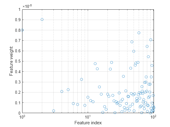
Plot the feature weights. The weights of the irrelevant features should be very close to zero.
semilogx(ncaMdl.FeatureWeights,"o")
xlabel("Feature index")
ylabel("Feature weight")
grid on
Predict the classes using the NCA model and compute the confusion matrix.
ypred = predict(ncaMdl,X);
confusionchart(y,ypred)
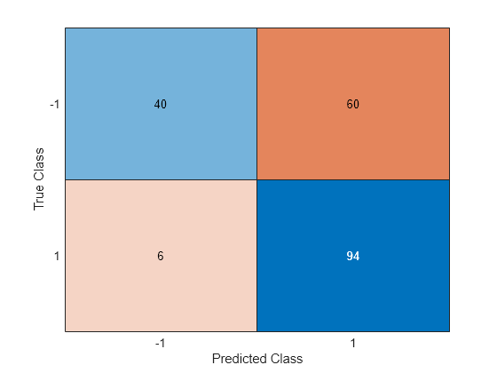
The confusion matrix shows that 40 of the data that are in class –1 are predicted as belonging to class –1, and 60 of the data from class –1 are predicted to be in class 1. Similarly, 94 of the data from class 1 are predicted to be from class 1, and 6 of them are predicted to be from class –1. The prediction accuracy for class –1 is not good.
All weights are very close to zero, which indicates that the value of used in training the model is too large. When , all features weights approach to zero. Hence, it is important to tune the regularization parameter in most cases to detect the relevant features.
Use five-fold cross-validation to tune for feature selection by using fscnca. Tuning means finding the value that will produce the minimum classification loss. To tune using cross-validation:
1. Partition the data into five folds. For each fold, cvpartition assigns four-fifths of the data as a training set and one-fifth of the data as a test set. Again for each fold, cvpartition creates a stratified partition, where each partition has roughly the same proportion of classes.
cvp = cvpartition(y,"KFold",5);
numtestsets = cvp.NumTestSets;
lambdavalues = linspace(0,2,20)/length(y);
lossvalues = zeros(length(lambdavalues),numtestsets);
2. Train the neighborhood component analysis (NCA) model for each value using the training set in each fold.
3. Compute the classification loss for the corresponding test set in the fold using the NCA model. Record the loss value.
4. Repeat this process for all folds and all values.
for i = 1:length(lambdavalues)
    for k = 1:numtestsets

        % Extract the training set from the partition object
        Xtrain = X(cvp.training(k),:);
        ytrain = y(cvp.training(k),:);

        % Extract the test set from the partition object
        Xtest  = X(cvp.test(k),:);
        ytest  = y(cvp.test(k),:);

        % Train an NCA model for classification using the training set
        ncaMdl = fscnca(Xtrain,ytrain,FitMethod="exact", ...
            Solver="lbfgs",Lambda=lambdavalues(i));

        % Compute the classification loss for the test set using the NCA
        % model
        lossvalues(i,k) = loss(ncaMdl,Xtest,ytest, ...
            LossFunction="quadratic");

    end
end
Plot the average loss values of the folds versus the values. If the value that corresponds to the minimum loss falls on the boundary of the tested values, the range of values should be reconsidered.
plot(lambdavalues,mean(lossvalues,2),"o-")
xlabel("Lambda values")
ylabel("Loss values")
grid on
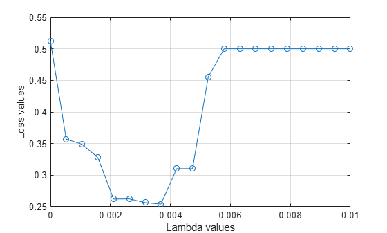
Find the value that corresponds to the minimum average loss.
[~,idx] = min(mean(lossvalues,2)); % Find the index
bestlambda = lambdavalues(idx) % Find the best lambda value
bestlambda =
0.0037
Fit the NCA model to all of the data using the best value. Use the LBFGS solver and display the convergence information.
ncaMdl = fscnca(X,y,FitMethod="exact",Verbose=1, ...
    Solver="lbfgs",Lambda=bestlambda);
 o Solver = LBFGS, HessianHistorySize = 15, LineSearchMethod = weakwolfe

|====================================================================================================|
|   ITER   |   FUN VALUE   |  NORM GRAD  |  NORM STEP  |  CURV  |    GAMMA    |    ALPHA    | ACCEPT |
|====================================================================================================|
|        0 | -1.246913e-01 |   1.231e-02 |   0.000e+00 |        |   4.873e+01 |   0.000e+00 |   YES  |
|        1 | -3.411330e-01 |   5.717e-03 |   3.618e+00 |    OK  |   1.068e+02 |   1.000e+00 |   YES  |
|        2 | -5.226111e-01 |   3.763e-02 |   8.252e+00 |    OK  |   7.825e+01 |   1.000e+00 |   YES  |
|        3 | -5.817731e-01 |   8.496e-03 |   2.340e+00 |    OK  |   5.591e+01 |   5.000e-01 |   YES  |
|        4 | -6.132632e-01 |   6.863e-03 |   2.526e+00 |    OK  |   8.228e+01 |   1.000e+00 |   YES  |
|        5 | -6.135264e-01 |   9.373e-03 |   7.341e-01 |    OK  |   3.244e+01 |   1.000e+00 |   YES  |
|        6 | -6.147894e-01 |   1.182e-03 |   2.933e-01 |    OK  |   2.447e+01 |   1.000e+00 |   YES  |
|        7 | -6.148714e-01 |   6.392e-04 |   6.688e-02 |    OK  |   3.195e+01 |   1.000e+00 |   YES  |
|        8 | -6.149524e-01 |   6.521e-04 |   9.934e-02 |    OK  |   1.236e+02 |   1.000e+00 |   YES  |
|        9 | -6.149972e-01 |   1.154e-04 |   1.191e-01 |    OK  |   1.171e+02 |   1.000e+00 |   YES  |
|       10 | -6.149990e-01 |   2.922e-05 |   1.983e-02 |    OK  |   7.365e+01 |   1.000e+00 |   YES  |
|       11 | -6.149993e-01 |   1.556e-05 |   8.354e-03 |    OK  |   1.288e+02 |   1.000e+00 |   YES  |
|       12 | -6.149994e-01 |   1.147e-05 |   7.256e-03 |    OK  |   2.332e+02 |   1.000e+00 |   YES  |
|       13 | -6.149995e-01 |   1.040e-05 |   6.781e-03 |    OK  |   2.287e+02 |   1.000e+00 |   YES  |
|       14 | -6.149996e-01 |   9.015e-06 |   6.265e-03 |    OK  |   9.974e+01 |   1.000e+00 |   YES  |
|       15 | -6.149996e-01 |   7.763e-06 |   5.206e-03 |    OK  |   2.919e+02 |   1.000e+00 |   YES  |
|       16 | -6.149997e-01 |   8.374e-06 |   1.679e-02 |    OK  |   6.878e+02 |   1.000e+00 |   YES  |
|       17 | -6.149997e-01 |   9.387e-06 |   9.542e-03 |    OK  |   1.284e+02 |   5.000e-01 |   YES  |
|       18 | -6.149997e-01 |   3.250e-06 |   5.114e-03 |    OK  |   1.225e+02 |   1.000e+00 |   YES  |
|       19 | -6.149997e-01 |   1.574e-06 |   1.275e-03 |    OK  |   1.808e+02 |   1.000e+00 |   YES  |

|====================================================================================================|
|   ITER   |   FUN VALUE   |  NORM GRAD  |  NORM STEP  |  CURV  |    GAMMA    |    ALPHA    | ACCEPT |
|====================================================================================================|
|       20 | -6.149997e-01 |   5.764e-07 |   6.765e-04 |    OK  |   2.905e+02 |   1.000e+00 |   YES  |

         Infinity norm of the final gradient = 5.764e-07
              Two norm of the final step     = 6.765e-04, TolX   = 1.000e-06
Relative infinity norm of the final gradient = 5.764e-07, TolFun = 1.000e-06
EXIT: Local minimum found.
Plot the feature weights.
semilogx(ncaMdl.FeatureWeights,"o")
xlabel("Feature index")
ylabel("Feature weight")
grid on
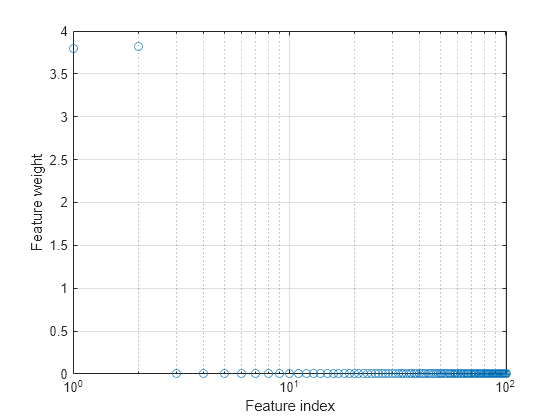
fscnca correctly figures out that the first two features are relevant and that the rest are not. The first two features are not individually informative, but when taken together result in an accurate classification model.
Predict the classes using the new model and compute the accuracy.
ypred = predict(ncaMdl,X);
confusionchart(y,ypred)
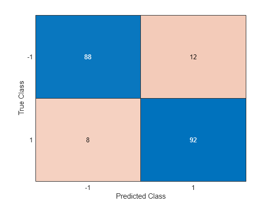
Confusion matrix shows that prediction accuracy for class –1 has improved. 88 of the data from class –1 are predicted to be from –1, and 12 of them are predicted to be from class 1. Additionally, 92 of the data from class 1 are predicted to be from class 1, and 8 of them are predicted to be from class –1.
References
[1] Yang, W., K. Wang, W. Zuo. "Neighborhood Component Feature Selection for High-Dimensional Data." Journal of Computers. Vol. 7, Number 1, January, 2012.
Input Arguments
Output Arguments
Version History
Introduced in R2016b
See Also
FeatureSelectionNCAClassification | predict | fscnca | refit | selectFeatures