Burr Type XII Distribution
Definition
The Burr type XII distribution is a three-parameter family of distributions on the positive real line. The cumulative distribution function (cdf) of the Burr distribution is
where c and k are the shape parameters and α is the scale parameter. The probability density function (pdf) is
The density of the Burr type XII distribution is L-shaped if c ≤ 1 and unimodal, otherwise.
Background
Burr distribution was first discussed by Burr (1942) as a two-parameter family. An additional scale parameter was introduced by Tadikamalla (1980). It is a flexible distribution family that can express a wide range of distribution shapes. The Burr distribution includes, overlaps, or has as a limiting case, many commonly used distributions such as gamma, lognormal, loglogistic, bell-shaped, and J-shaped beta distributions (but not U-shaped). Some compound distributions also correspond to the Burr distribution. For example, compounding a Weibull distribution with a gamma distribution for its scale parameter results in a Burr distribution. Similarly, compounding an exponential distribution with a gamma distribution for its rate parameter, 1/μ, also yields a Burr distribution. The Burr distribution also has two asymptotic limiting cases: Weibull and Pareto Type I.
The Burr distribution can fit a wide range of empirical data. Different values of its parameters cover a broad set of skewness and kurtosis. Hence, it is used in various fields such as finance, hydrology, and reliability to model a variety of data types. Examples of data modeled by the Burr distribution are household income, crop prices, insurance risk, travel time, flood levels, and failure data.
The survival and hazard functions of Burr type XII distribution are, respectively,
and
If c > 1, the hazard function h(x) is non-monotonic with a mode at x = α(c – 1)1/c.
Parameters
The three-parameter Burr distribution is defined by its scale parameter α and
shape parameters c and k. You can estimate the
parameters using mle or fitdist. Both
functions support censored data for Burr distribution.
Generate sample data from a Burr distribution with scale parameter 0.5 and shape parameters 2 and 5.
rng('default')
R = random('burr',0.5,2,5,1000,1);
Estimate the parameters and the confidence intervals.
[phat,pci] = mle(R,'distribution','burr')
phat =

    0.4154    2.1217    4.0550


pci =

    0.2985    1.9560    2.4079
    0.5782    2.3014    6.8288
The three-parameter Burr distribution converges asymptotically to one of the two limiting forms as its parameters diverge:
If k→0, c→∞, ck = λ, then the Burr distribution reduces to a two-parameter Pareto distribution with the cdf
If k→∞, α→∞, α/k1/c = θ, then the Burr distribution reduces to a two-parameter Weibull distribution with the cdf
If mle or fitdist detects such divergence,
it returns an error message, but informs you of the limiting distribution and
corresponding parameter estimates for that distribution.
Fit a Burr Distribution and Draw the cdf
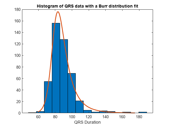
This example shows how to fit a Burr distribution to data, draw the cdf, and construct a histogram with a Burr distribution fit.
1. Load the sample data.
load arrhythmiaThe fifth column in X contains a measurement obtained from electrocardiograms, called QRS duration.
2. Fit a Burr distribution to the QRS duration data, and get the parameter estimates.
PD = fitdist(X(:,5),'burr');PD has the maximum likelihood estimates of the Burr distribution parameters in the property Param. The estimates are α = 80.4515, = 18.9251, = 0.4492.
3. Plot the cdf of the QRS duration data.
QRScdf=cdf('burr',sortrows(X(:,5)),80.4515,18.9251,0.4492);
plot(sortrows(X(:,5)),QRScdf)
title('QRS duration data')
xlabel('QRS Duration')

4. Draw the histogram of QRS duration data with 15 bins and the pdf of the Burr distribution fit.
histfit(X(:,5),15,'burr')
title('Histogram of QRS data with a Burr distribution fit')
xlabel('QRS Duration')

Compare Lognormal and Burr Distribution pdfs
Compare the lognormal pdf to the Burr pdf using income data generated from a lognormal distribution.
Generate the income data.
rng('default') % For reproducibility
y = random('Lognormal',log(25000),0.65,[500,1]);
Fit a Burr distribution.
pd = fitdist(y,'burr')pd =
BurrDistribution
Burr distribution
alpha = 26007.2 [21165.5, 31956.4]
c = 2.63743 [2.3053, 3.0174]
k = 1.09658 [0.775479, 1.55064]
Plot both the Burr and lognormal pdfs of income data on the same figure.
p_burr = pdf(pd,sortrows(y));
p_lognormal = pdf('Lognormal',sortrows(y),log(25000),0.65);
plot(sortrows(y),p_burr,'-',sortrows(y),p_lognormal,'-.')
title('Burr and Lognormal pdfs Fit to Income Data')
legend('Burr Distribution','Lognormal Distribution')

Burr pdf for Various Parameters
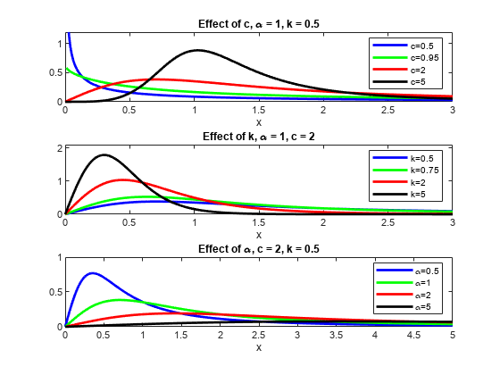
This example shows how to create a variety of shapes for probability density functions of the Burr distribution.
X = 0:0.01:5;
c = [0.5 0.95 2 5];
k = [0.5 0.75 2 5];
alpha = [0.5 1 2 5];
colors = ['b';'g';'r';'k']';

figure
for i = 1:1:4
pdf1(i,:) = pdf('burr',X,1,c(i),0.5);
pdf2(i,:) = pdf('burr',X,1,2,k(i));
pdf3(i,:) = pdf('burr',X,alpha(i),2,0.5);

axC = subplot(3,1,1);
pC(i) = plot(X,pdf1(i,:),colors(i),'LineWidth',2);
title('Effect of c, \alpha = 1, k = 0.5'),xlabel('x')
hold on

axK = subplot(3,1,2);
pK(i) = plot(X,pdf2(i,:),colors(i),'LineWidth',2);
title('Effect of k, \alpha = 1, c = 2'),xlabel('x')
hold on

axAlpha = subplot(3,1,3);
pAlpha(i) = plot(X,pdf3(i,:),colors(i),'LineWidth',2);
title('Effect of \alpha, c = 2, k = 0.5'),xlabel('x')
hold on
end

set(axC,'XLim',[0 3],'YLim',[0 1.2]);
set(axK,'XLim',[0 3],'YLim',[0 2.1]);
set(axAlpha,'XLim',[0 5],'YLim',[0 1]);

legend(axC,'c=0.5','c=0.95','c=2','c=5');
legend(axK,'k=0.5','k=0.75','k=2','k=5');
legend(axAlpha,'\alpha=0.5','\alpha=1','\alpha=2','\alpha=5');

This figure illustrates how the shape and scale of the Burr distribution changes for different values of its parameters.
Survival and Hazard Functions of Burr Distribution
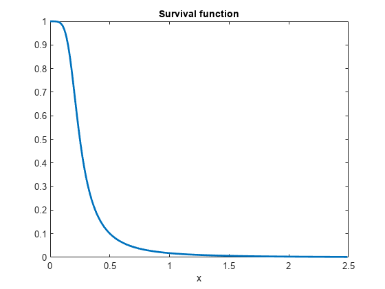
This example shows how to find and plot the survival and hazard functions for a sample coming from a Burr distribution.
Generate the data.
X = 0:0.015:2.5;
Evaluate the pdf and cdf of data in X.
Xpdf = pdf('burr',X,0.2,5,0.5);
Xcdf = cdf('burr',X,0.2,5,0.5);
Evaluate and plot the survival function of data in X.
S = 1.-Xcdf; % survival function
plot(X,S,'LineWidth',2)
title('Survival function')
xlabel('x')

Evaluate and plot the hazard function of data in X.
H = Xpdf./S; % hazard function
plot(X,H,'r','LineWidth',2)
title('Hazard function')
xlabel('x')

Divergence of Parameter Estimates
This example shows how to interpret the display when the parameter estimates diverge when fitting a Burr distribution to input data.
1. Generate sample data from the Weibull distribution with parameters 0.5 and 2.
rng('default') % for reproducibility
X = wblrnd(0.5,2,100,1);
2. Fit a Burr distribution.
PD = fitdist(X,'burr');Error using addburr>burrfit (line 566)
The data are not fit by a Burr distribution with finite parameters.
The maximum likelihood fit is provided by the k->Inf, alpha->Inf
limiting form of the Burr distribution: a Weibull distribution
with the parameters below.
a (scale): 0.476817
b (shape): 1.96219
Error in prob.BurrDistribution.fit (line 246)
p = burrfit(x,0.05,cens,freq,opt);
Error in fitdist>localfit (line 238)
pd = feval(fitter,x,'cens',c,'freq',f,varargin{:});
Error in fitdist (line 185)
pd = localfit(dist,fitter,x,cens,freq,args{:});The error message tells you that the Weibull family seems to fit the data better and gives you the parameter estimates from a Weibull fit. You can use those estimates directly. If you need covariance estimates for the parameters or other information about the fit, you can refit a Weibull distribution to the data.
3. Fit a Weibull distribution to the data and find the confidence intervals for the parameter estimates.
PD = fitdist(X,'weibull');
paramci(PD)
ans =
0.4291 1.6821
0.5298 2.2890These are the 95% confidence intervals of the parameter estimates for the Weibull distribution fit.
References
[1] Burr, Irving W. “Cumulative frequency functions.” The Annals of Mathematical Statistics, Vol. 13, Number 2, 1942, pp. 215–232.
[2] Tadikamalla, Pandu R. “A look at the Burr and related distributions.” International Statistical Review, Vol. 48, Number 3, 1980, pp. 337–344.
[3] Rodriguez, Robert N. “A guide to the Burr type XII distributions.” Biometrika, Vol. 64, Number 1, 1977, pp. 129–134.
[4] Al-Hussaini, Essam K. “A characterization of the Burr type XII distribution”. Appl. Math. Lett. Vol. 4, Number 1, 1991, pp. 59–61.
[5] Grammig, Joachim and Kai-Oliver Maurer. “Non-monotonic hazard functions and the autoregressive conditional duration model.” Econometrics Journal, Vol. 3, 2000, pp. 16–38.