Specify Custom Linearizations for Simulink Blocks

This example shows how to specify the linearization of a Simulink® block or subsystem.

In Simulink Control Design™ software, linearization provides a linear approximation of a Simulink model using an exact linearization approach. This linearization is valid in a small region around a given operating point. This approach works well for most Simulink models. However, in some cases, you must modify the exact linearization approach to take into account the effects of discontinuities or approximate the dynamics of derivative or delay action. Many built-in Simulink blocks, such as Saturation or Dead Zone blocks, provide a Treat as gain when linearizing parameter to control this behavior. For blocks or subsystems that cannot be linearized, it can be necessary to specify a linearization. In this example, you specify a custom linearization for a subsystem to approximate the linearization of a PWM signal.

Linearize a Model with a PWM Generation Subsystem

The scdpwm model contains a Voltage to PWM subsystem that models a PWM signal, which then enters a plant model.

mdl = 'scdpwm';
open_system(mdl)

When you linearize this model using the standard configuration, the resulting linear model has a gain of zero.

io = getlinio(mdl);
sys = linearize(mdl,io)

sys =
 
  D = 
                Step
   Plant Model     0
 
Static gain.

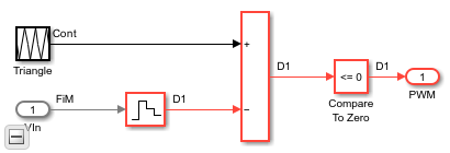
The Voltage to PWM/Compare To Zero block causes this linearization to be zero.

pwmblk = 'scdpwm/Voltage to PWM';
open_system(pwmblk)

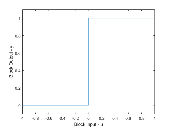
The linearization is zero because the block represents a pure discontinuous nonlinearity.

u = [-1:0.1:0,0:0.1:1];
y = [zeros(11,1);ones(11,1)];
plot(u,y)
xlabel('Block Input - u')
ylabel('Block Output - y')
ylim([-0.1 1.1])

Specify a Custom Linearization for the PWM Subsystem

With Simulink Control Design software, you can control the linearization of the blocks in a Simulink model. You can specify the linearization of a block using:

• Matrices

• Linear time invariant models, such as transfer functions or state-space models

• Uncertain parameters or state-space models (requires Robust Control toolbox™ software)

In this example, the PWM subsystem contains a time delay

This time delay accounts for the duty cycle frequency of the PWM signal which is 100 Hz. To specify the delay for the Voltage to PWM subsystem, first select the block. Then, on the Apps tab, click Linearization Manager.

On the Linearization tab, click Specify Block Linearization. Then, in the Block Linearization Specification dialog box, perform the following steps.

1. Select the Specify block linearization using one of the following parameter.

2. In the drop-down box, select MATLAB Expression.

3. Specify the linearization using the expression ss(1,'OutputDelay',1/100).

The following code is equivalent to entering the delay into the Block Linearization Specification dialog box.

set_param(pwmblk,'SCDEnableBlockLinearizationSpecification','on');
rep = struct('Specification','ss(1,''OutputDelay'',1/100)',...
             'Type','Expression',...
             'ParameterNames','',...
             'ParameterValues','');
set_param(pwmblk,'SCDBlockLinearizationSpecification',rep);

Create a continuous-time linear model of the system.

opt = linearizeOptions('SampleTime',0);
sys = linearize(mdl,io,opt);

The linearized model, which includes the specified subsystem linearization, now gives the expected result.

sys = zpk(sys)

sys =
 
  From input "Step" to output "Plant Model":
                       1
  exp(-0.01*s) * -------------
                 (s^2 + s + 1)
 
Continuous-time zero/pole/gain model.

Compare the Linearization and Simulation

You can compare the linearization of the model to an estimated frequency response of the model using a frest.createStep input signal.

The linearization you specified for the Voltage to PWM subsystem affects only linearization and not model simulation. Therefore, you do not need to remove the linearization specification before you estimate the frequency response.

Create an input signal and estimate the frequency response of the model.

instep = frest.createStep('Ts',1/10000,'StepTime',1,...
                          'StepSize',1e-1,'FinalTime',15);
[sysf,simoutstep] = frestimate(mdl,io,instep);

Compare the linearized model with the simulation results from the estimated model.

frest.simCompare(simoutstep,sys,instep)
legend('Linearization with PWM Subsystem Specification',...
            'Simulated Step Response','Location','East')

The linearization accurately represents the dynamics of the estimated system.

Other Applications for Custom Linearizations

Block linearization specification is not limited to linear time-invariant models. If you have Robust Control Toolbox™ software, you can specify uncertain parameters and uncertain state-space (USS) models for blocks in a model. The resulting linearization is then an uncertain model. The example Linearization of Simulink Models with Uncertainty (Robust Control Toolbox) shows how to compute a linearization with uncertainty.

You can also perform analysis of models with discrete controllers and continuous plant dynamics in the continuous domain. For more details, see Model Computational Delay and Sampling Effects.

Close the Simulink model.

bdclose(mdl)