주요 콘텐츠

plot

R2026b

Plot measured and simulated impedance for profile at specific index

Since R2025a

Description

plot(eisfom) plots the measured and simulated impedances for the first profile inside the EISModel object, eisfom.

example

plot(eisfom,profileId) plots the measured and simulated impedance for the profile at the index specified by profileId inside the EISModel object, eisfom.

plot(___,Name=Value) also specifies options using one or more name-value arguments.

chart = plot(___) returns a ImpedanceVerificationChart object.

Examples

collapse all

This example shows how to plot the measured and simulated impedance for all profiles inside an EISModel object.

Open the DownloadBatteryEISData example and load the required electrochemical impedance spectroscopy (EIS) data. This data has been generated from a battery with a nominal capacity of 30/1000 A*Hr at a temperature of 25 °C. This data consists of a 500-by-3 matrix of doubles. The columns of the matrix refer to the frequency, real impedance, and imaginary impedance values, respectively.

openExample("simscapebattery/DownloadBatteryEISDataExample")
load("generatedEISData.mat")

Fit the EIS data to a fractional-order equivalent circuit model. To fit the data and create an EISModel object, use the fitEISModel function.

eisfom = fitEISModel(eisData);

Analyze how the function performed the fit on the frequency model by using the plot function. This plot shows the simulated data against the measured data, where the X-axis represents the real part of the impedance and the Y-axis represents the imaginary part of the impedance.

plot(eisfom,Parent=figure,DisplayMode="Nyquist")

Plot of the simulated and measured impedance data with a Nyquist display.

You can also plot the imaginary impedance over the log frequency by setting the DisplayMode argument to "ImagZ(f)".

plot(eisfom,Parent=figure,DisplayMode="ImagZ(f)")
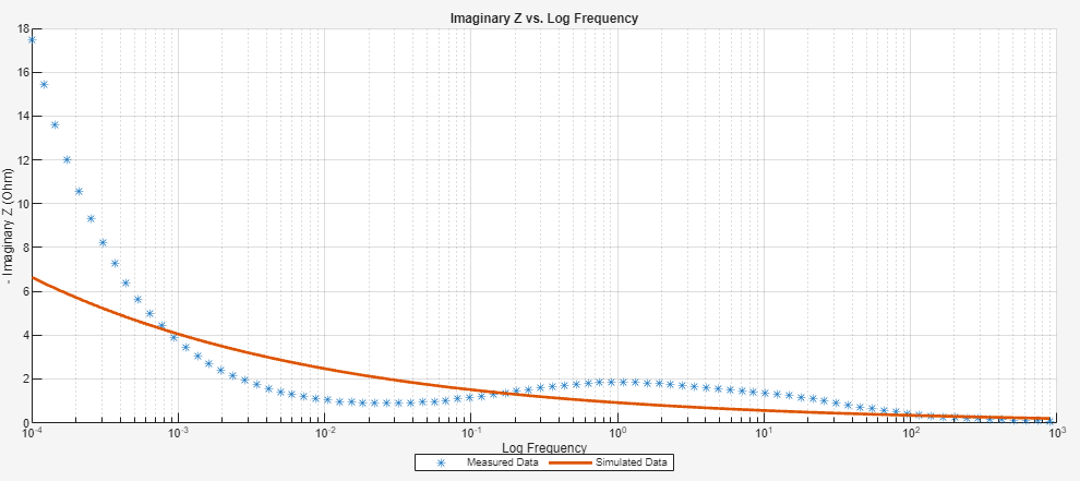
Plot of the simulated and measured impedance data with a ImagZ(f) display.

To plot both figures, set the DisplayMode argument to "Nyq_ImagZ(f)".
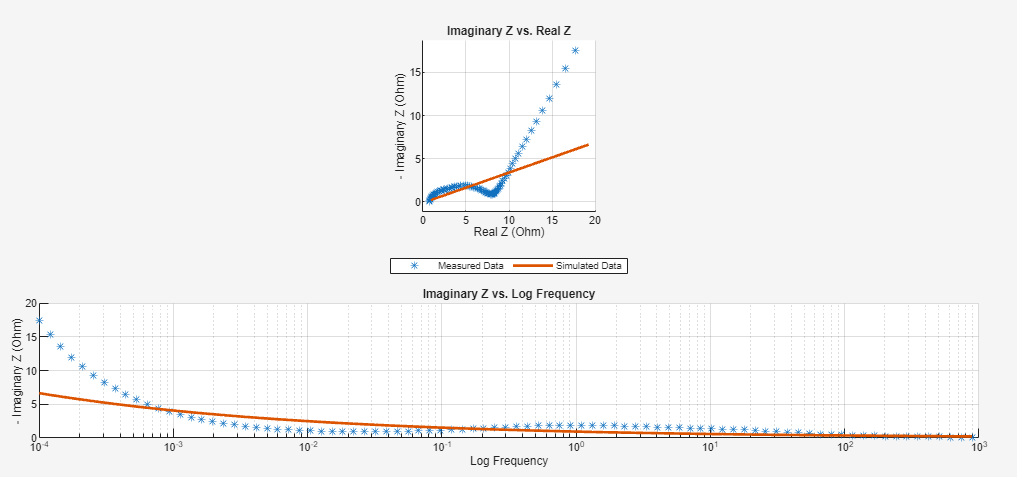
Plot of the simulated and measured impedance data with both Nyquist and ImagZ(f) displays.

Input Arguments

collapse all

Fractional-order equivalent circuit model used to plot the simulated impedance for the specified tabulated profile, specified as an EISModel object.

Indices of the tabulated profile inside the ImpedanceData and ParameterSummary property tables of the EISModel object, specified as a scalar.

Data Types: double

Name-Value Arguments

collapse all

Specify optional pairs of arguments as Name1=Value1,...,NameN=ValueN, where Name is the argument name and Value is the corresponding value. Name-value arguments must appear after other arguments, but the order of the pairs does not matter.

Example: plotPulse(myTest,indices,PlottingQuadrant="fourth")

Measured impedance data, specified as a matrix with three columns. The first column contains the frequency, the second column contains the real part of the impedance, and the third column contains the imaginary part of the impedance.

Simulated impedance data, specified as a matrix with three columns. The first column contains the frequency, the second column contains the real part of the impedance, and the third column contains the imaginary part of the impedance.

Aspect ratio for the Nyquist chart, specified as a vector of three positive elements.

Quadrant in which to plot the impedance values, specified as "first" or "fourth".

Display mode of the chart, specified as "Nyquist", "ImagZ(f)", or "Nyq_ImagZ(f)".

The plot function also accepts all properties of the ComponentContainer class as name-value arguments. For a list of these properties, see matlab.ui.componentcontainer.ComponentContainer.

Output Arguments

collapse all

Chart for visualizing the measured and simulated impedance of specified tabulated pulse, returned as a ImpedanceVerificationChart object.

Version History

Introduced in R2025a