settlingtime
Settling time for bilevel waveform
Syntax
Description
s = settlingtime(x,d)d. To determine the transitions, the
settlingtime function estimates the state levels of the
input waveform by a histogram method and identifies all regions that cross the
upper-state boundary of the low state and the lower-state boundary of the high state.
Note
If for any transition, the level of the waveform does not remain within
the lower and upper tolerance boundaries, the requested duration is not
present, or an intervening transition is detected,
settlingtime marks the corresponding element in
s as NaN. For cases in which
settlingtime returns a NaN, see
Settle Seek Duration.
[
returns the settling times, levels, and corresponding sample instants with
additional options specified by one or more name-value arguments. You can specify an
input combination from any of the previous syntaxes.s,slev,sinst]
= settlingtime(___,Name,Value)
settlingtime(___) plots the signal and darkens
the regions of each transition where settling time is computed. The plot marks the
location of the settling time of each transition, the mid-crossings, and the
associated reference levels. The plot also displays the state levels with the
corresponding lower and upper tolerance boundaries.
Examples
Determine the settling point and corresponding waveform value for a bilevel waveform. Specify a settle-seek duration of 10 seconds.
load('transitionex.mat', 'x')
[s,slev,sinst] = settlingtime(x,10);
Plot the waveform and annotate the settling point.
settlingtime(x,10)
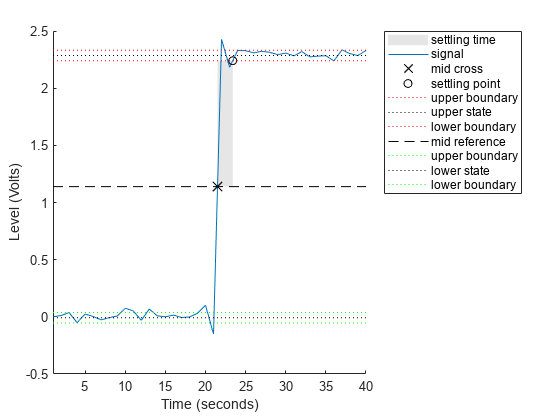
ans =
1.8901
Determine the settling points for a three-transition bilevel waveform. The data are sampled at 4 MHz. Specify a settle-seek duration of one microsecond.
load('transitionex.mat','x')
y = [x; fliplr(x)];
fs = 4e6;
t = 0:1/fs:(length(y)*1/fs)-1/fs;

[s,slev,sinst] = settlingtime(y,fs,1e-6);
Plot the waveform and annotate the settling points.
settlingtime(y,fs,1e-6)
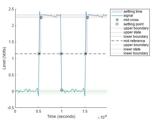
ans = 3×1
10-6 ×

    0.4725
    0.1181
    0.4725
Input Arguments
Name-Value Arguments
Output Arguments
More About
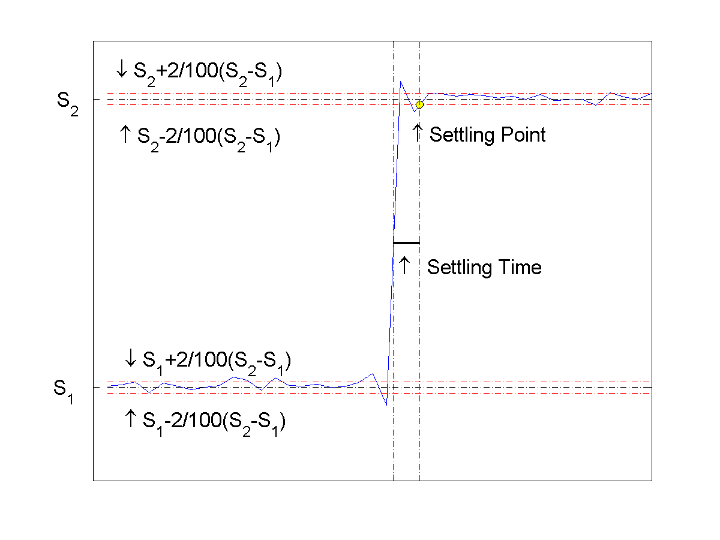
The settling time is the time after the mid-reference level instant when the signal crosses into and remains in the 2%-tolerance region around the state level. The settling time is illustrated in this figure, where the low- and high-state levels are the dashed black lines, the 2% tolerances above and below the state levels are shown by the red dashed lines, and the settling time is indicated by the yellow circle.
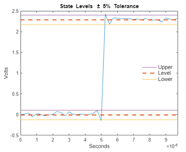
You can specify lower- and upper-state boundaries for each state level. Define the boundaries as the state level plus or minus a scalar multiple of the difference between the high state and the low state. To provide a useful tolerance region, specify the scalar as a small number such as 2/100 or 3/100. In general, the region for the low state is defined as
where is the low-state level and is the high-state level. Replace the first term in the equation with to obtain the tolerance region for the high state.
This figure shows lower and upper 5% state boundaries (tolerance regions) for a positive-polarity bi-level waveform. The thick dashed lines indicate the estimated state levels.
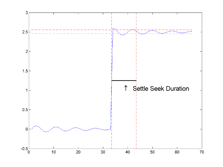
The settle seek duration defines the interval of time after the mid-reference
level instant that settlingtime looks for a settling point. If
settlingtime does not find a settling point within the
settle seek duration, settlingtime returns
NaN for the settling time. This figure illustrates a settle
seek duration of 10 samples.
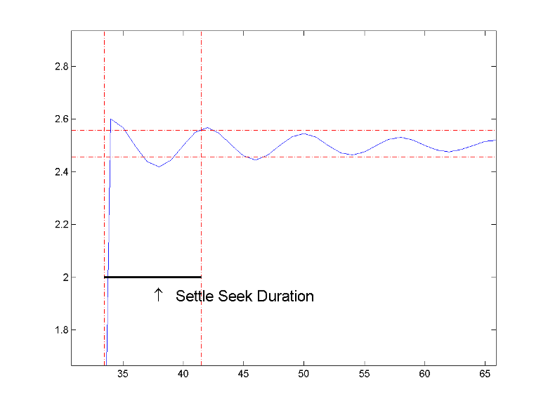
The settlingtime function may fail to find a settling point in the
specified settle seek duration if any one of these conditions occurs:
The last waveform value in the settle seek interval is not within the upper- and lower-state boundaries determined by the specified tolerance. This figure illustrates this condition for a settle seek duration of 8 samples and a 2% tolerance region. The last sample in the settle seek interval exceeds the upper state boundary. In this example, reducing or increasing the settle seek duration can result in a valid settling time.
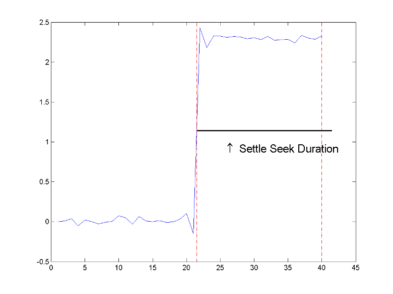
There is an insufficient number of waveform samples for the specified settle seek duration. This figure illustrates this condition for a settle seek duration of 20 samples. The settle seek duration extends beyond the final sample of the waveform.
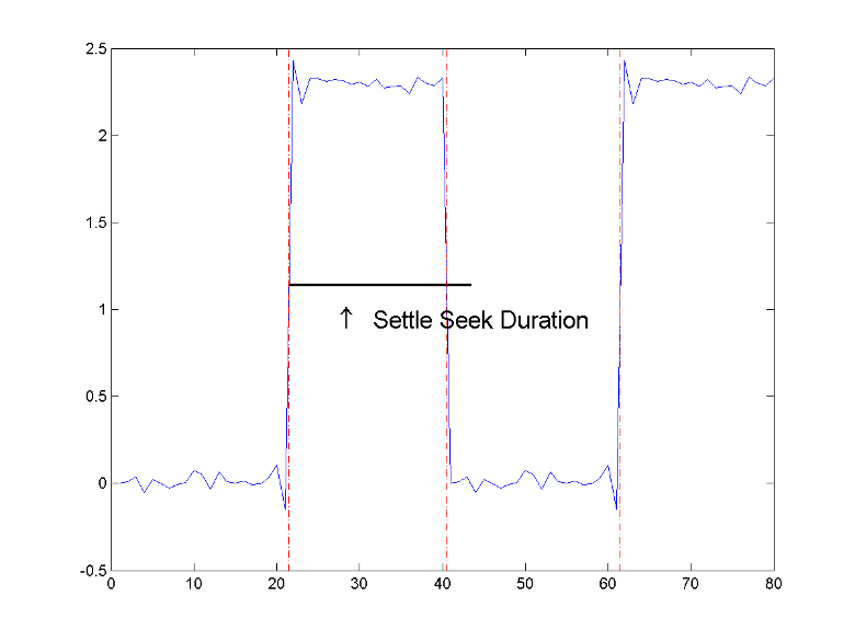
An intervening transition is detected before the end of the specified settle seek duration. This figure illustrates this condition for a settle seek duration of 22 samples. An intervening transition is detected before the end of the 22–sample settle seek duration.
References
[1] IEEE® Standard on Transitions, Pulses, and Related Waveforms, IEEE Standard 181, 2003, pp. 23–24.
Extended Capabilities
Version History
Introduced in R2012a
See Also
falltime | midcross | pulsewidth | risetime | statelevels