이 번역 페이지는 최신 내용을 담고 있지 않습니다. 최신 내용을 영문으로 보려면 여기를 클릭하십시오.
위성군에 대한 커버리지 지도
이 예제에서는 위성 시나리오와 2차원 지도를 사용하여 관심 영역에 대한 커버리지 지도를 표시하는 방법을 보여줍니다. 위성에 대한 커버리지 지도에는 어떤 영역 내의 지상 수신기로의 다운링크에서 발생하는 그 영역 전체의 수신 전력이 포함됩니다.
Mapping Toolbox™의 매핑 기능과 Satellite Communications Toolbox의 위성 시나리오 기능을 결합하면 등고선이 그려진 커버리지 지도를 만들고 등고선 데이터를 시각화 및 분석에 사용할 수 있습니다. 이 예제에서는 다음을 수행하는 방법을 보여줍니다.
지상국 수신기의 그리드가 포함된 위성 시나리오를 사용하여 커버리지 지도 데이터를 계산합니다.
axesm-기반 지도와 지도 좌표축을 포함한 다양한 지도 표시를 사용하여 커버리지 지도를 봅니다.다른 관심 시간의 커버리지 지도를 계산하고 확인합니다.
시나리오를 만들고 시각화하기
위성 시나리오와 뷰어를 만듭니다. 시나리오의 시작 날짜와 지속 시간(1시간)을 지정합니다.
startTime = datetime(2023,2,21,18,0,0);
stopTime = startTime + hours(1);
sampleTime = 60; % seconds
sc = satelliteScenario(startTime,stopTime,sampleTime);
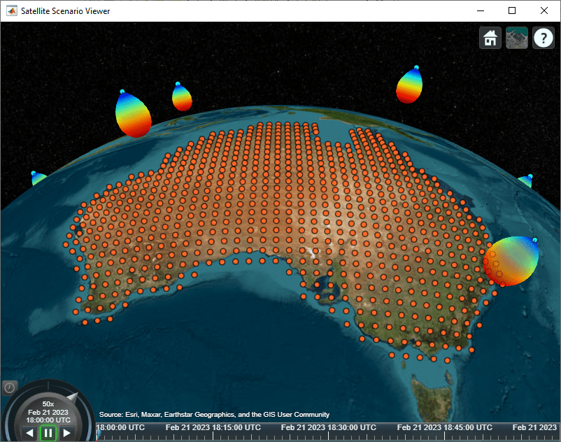
viewer = satelliteScenarioViewer(sc,ShowDetails=false);위성군 추가하기
2018년에서 2019년 사이에 발사된 Iridium NEXT 위성 네트워크[1]에는 다음과 같은 66개의 활성 LEO 위성이 포함되어 있습니다.
6개의 궤도면으로 이루어져 있으며 경사각은 약 86.6도이고 궤도면 간 RAAN 차이는 약 30도입니다[1].
각 궤도면에는 11개의 위성이 있으며 위성 간 진근점 이각(true anomaly) 차이는 약 32.7도입니다[1].
시나리오에 활성 Iridium NEXT 위성을 추가합니다. Iridium 네트워크의 위성에 대한 궤도 요소를 만들고 위성을 만듭니다.
numSatellitesPerOrbitalPlane = 11;
numOrbits = 6;

orbitIdx = repelem(1:numOrbits,1,numSatellitesPerOrbitalPlane);
planeIdx = repmat(1:numSatellitesPerOrbitalPlane,1,numOrbits);

RAAN = 180*(orbitIdx-1)/numOrbits;
trueanomaly = 360*(planeIdx-1 + 0.5*(mod(orbitIdx,2)-1))/numSatellitesPerOrbitalPlane;
semimajoraxis = repmat((6371 + 780)*1e3,size(RAAN)); % meters
inclination = repmat(86.4,size(RAAN)); % degrees
eccentricity = zeros(size(RAAN)); % degrees
argofperiapsis = zeros(size(RAAN)); % degrees

iridiumSatellites = satellite(sc,...
    semimajoraxis,eccentricity,inclination,RAAN,argofperiapsis,trueanomaly,...
    Name="Iridium " + string(1:66)');
Aerospace Toolbox™ 라이선스가 있는 경우 walkerStar (Aerospace Toolbox) 함수를 사용하여 Iridium 위성군을 만들 수도 있습니다.
호주 주변 관심 영역 정의하기
호주를 둘러싼 AOI(관심 영역)를 만들어 커버리지 지도를 계산할 준비를 합니다.
전 세계 육지 영역이 포함된 shapefile을 지리공간 테이블로서 작업 공간으로 읽어옵니다. 지리공간 테이블은 지리 좌표에서 다각형을 사용하여 육지 영역을 나타냅니다. 호주에 해당하는 다각형을 추출합니다.
landareas = readgeotable("landareas.shp");
australia = geocode("Australia",landareas);
호주 육지 영역을 중심으로 1도의 버퍼 영역을 포함하는 새로운 다각형을 지리 좌표에 만듭니다. 버퍼는 커버리지 지도 범위가 육지 영역을 포함하도록 해 줍니다.
bufwidth = 1; % degrees
aoi = buffer(australia.Shape,bufwidth);
AOI를 커버하는 지상국 그리드 추가하기
AOI를 커버하는 지상국 수신기 그리드의 신호 강도를 계산하여 커버리지 지도 데이터를 만듭니다. 위도-경도 좌표 그리드를 만들고 AOI 내 좌표를 선택하여 지상국 위치를 만듭니다.
AOI의 위도 제한과 경도 제한을 계산하고 간격을 도 단위로 지정합니다. 간격은 지상국 간의 거리를 결정합니다. 간격 값이 낮을수록 커버리지 지도 해상도가 향상되지만 계산 시간도 증가합니다.
[latlim, lonlim] = bounds(aoi);
spacingInLatLon = 1; % degrees
호주에 적합한 투영된 CRS(참조 좌표계)를 만듭니다. 투영된 CRS는 물리적 위치에 카테시안 x, y 지도 좌표를 할당하는 정보를 제공합니다. 람베르트 등각 원뿔 도법을 사용하는, 호주에 적합한 GDA2020 / GA LCC 투영된 CRS를 사용합니다.
proj = projcrs(7845);
데이터 그리드의 투영된 X-Y 지도 좌표를 계산합니다. 위도-경도 좌표 대신 투영된 X-Y 지도 좌표를 사용하여 그리드 위치 간 거리 변동을 줄입니다.
spacingInXY = deg2km(spacingInLatLon)*1000; % meters
[xlimits,ylimits] = projfwd(proj,latlim,lonlim);
R = maprefpostings(xlimits,ylimits,spacingInXY,spacingInXY);
[X,Y] = worldGrid(R);
그리드 위치를 위도-경도 좌표로 변환합니다.
[gridlat,gridlon] = projinv(proj,X,Y);
AOI 내 그리드 좌표를 선택합니다.
gridpts = geopointshape(gridlat,gridlon);
inregion = isinterior(aoi,gridpts);

gslat = gridlat(inregion);
gslon = gridlon(inregion);
해당 좌표에 지상국을 만듭니다.
gs = groundStation(sc,gslat,gslon);
송신기와 수신기 추가하기
위성에 송신기를 추가하고 지상국에 수신기를 추가하여 다운링크 모델링을 활성화합니다.
Iridium 위성군은 48빔 안테나를 사용합니다. 가우스 안테나 또는 사용자 지정 48빔 안테나를 선택합니다(Phased Array System Toolbox™ 필요). 가우스 안테나는 62.7도의 Iridium 반시야각[1]을 사용하여 48빔 안테나를 근사합니다. 안테나가 천저 방향을 향하도록 합니다.
fq = 1625e6; % Hz txpower = 20; % dBW antennaType ="Gaussian"; halfBeamWidth = 62.7; % degrees
가우스 안테나를 사용하는 위성 송신기를 추가합니다.
if antennaType == "Gaussian"
    lambda = physconst('lightspeed')/fq; % meters
    dishD = (70*lambda)/(2*halfBeamWidth); % meters
    tx = transmitter(iridiumSatellites, ...
        Frequency=fq, ...
        Power=txpower);
    gaussianAntenna(tx,DishDiameter=dishD);
end
사용자 지정 48빔 안테나를 사용하는 위성 송신기를 추가합니다. 헬퍼 함수 helperCustom48BeamAntenna는 예제에 지원 파일로 포함되어 있습니다.
if antennaType == "Custom 48-Beam"
    antenna = helperCustom48BeamAntenna(fq);
    tx = transmitter(iridiumSatellites, ...
        Frequency=fq, ...
        MountingAngles=[0,-90,0], ... % [yaw, pitch, roll] with -90 using Phased Array System Toolbox convention
        Power=txpower, ...
        Antenna=antenna);
end
지상국 수신기 추가하기
등방성 안테나를 사용하는 지상국 수신기를 추가합니다.
isotropic = arrayConfig(Size=[1 1]);
rx = receiver(gs,Antenna=isotropic);
위성 송신기 안테나 패턴을 시각화합니다. 시각화는 안테나의 천저 지향 방향을 보여줍니다.
pattern(tx,Size=500000);
래스터 커버리지 지도 데이터 계산하기
위성 시나리오 뷰어를 닫고 시나리오 시작 시간에 해당하는 커버리지 데이터를 계산합니다. satcoverage 헬퍼 함수는 그리딩된 커버리지 데이터를 반환합니다. 이 함수는 각 위성에 대해 시야 모양을 계산하고 위성 시야 내의 각 지상국 수신기에 대한 신호 강도를 계산합니다. 커버리지 데이터는 위성으로부터 수신되는 최대 신호 강도입니다.
delete(viewer)
maxsigstrength = satcoverage(gridpts,sc,startTime,inregion,halfBeamWidth);
axesm 기반 지도에 커버리지 시각화하기
호주에 해당하는 axesm 기반 지도에 래스터 커버리지 지도 데이터를 플로팅합니다. 지도 좌표축은 벡터 데이터 플로팅만 지원하므로 벡터 데이터와 래스터 데이터의 혼합 플로팅을 지원하는 axesm 기반 지도가 사용됩니다.
표시할 최소 전력 수준과 최대 전력 수준을 정의합니다.
minpowerlevel = -120; % dBm
maxpowerlevel = -106; % dBm
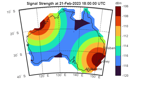
호주의 세계 지도를 만들고 래스터 커버리지 지도 데이터를 등고선 표시로 플로팅합니다.
figure
worldmap(latlim,lonlim)
mlabel south

colormap turbo
clim([minpowerlevel maxpowerlevel])
geoshow(gridlat,gridlon,maxsigstrength,DisplayType="contour",Fill="on")
geoshow(australia,FaceColor="none")

cBar = contourcbar;
title(cBar,"dBm");
title("Signal Strength at " + string(startTime) + " UTC")
시드니, 멜버른, 브리즈번 도시에 텍스트 레이블을 추가합니다. geocode 함수를 사용하여 각 도시의 좌표를 구합니다.
sydneyT = geocode("Sydney,Australia","city");
sydney = sydneyT.Shape;
melbourneT = geocode("Melbourne,Australia","city");
melbourne = melbourneT.Shape;
brisbaneT = geocode("Brisbane,Australia","city");
brisbane = brisbaneT.Shape;

textm(sydney.Latitude,sydney.Longitude,"Sydney")
textm(melbourne.Latitude,melbourne.Longitude,"Melbourne")
textm(brisbane.Latitude,brisbane.Longitude,"Brisbane")
커버리지 지도 등고선 계산하기
래스터 커버리지 지도 데이터의 등고선을 그려 커버리지 지도 등고선의 지리공간 테이블을 만듭니다. 각 커버리지 지도 등고선은 지리 좌표에 있는 다각형을 포함하는 지리공간 테이블에서 행으로 표현됩니다. 커버리지 지도 등고선은 시각화와 분석 모두에 사용할 수 있습니다.
levels = linspace(minpowerlevel,maxpowerlevel,8);
GT = contourDataGrid(gridlat,gridlon,maxsigstrength,levels,proj);
GT = sortrows(GT,"Power (dBm)");
disp(GT)
Shape Area (sq km) Power (dBm) Power Range (dBm)
____________ ____________ ___________ _________________
geopolyshape 8.5438e+06 -120 -120 -118
geopolyshape 8.2537e+06 -118 -118 -116
geopolyshape 5.5607e+06 -116 -116 -114
geopolyshape 3.6842e+06 -114 -114 -112
geopolyshape 2.2841e+06 -112 -112 -110
geopolyshape 1.1843e+06 -110 -110 -108
geopolyshape 3.8307e+05 -108 -108 -106
지도 좌표축에 커버리지 시각화하기
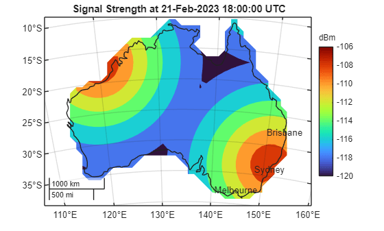
호주에 대한 지도 투영을 사용하여 지도 좌표축에 커버리지 지도 등고선을 플로팅합니다. 자세한 내용은 Choose a 2-D Map Display (Mapping Toolbox) 항목을 참조하십시오.
figure
newmap(proj)
hold on

colormap turbo
clim([minpowerlevel maxpowerlevel])
geoplot(GT,ColorVariable="Power (dBm)",EdgeColor="none")
geoplot(australia,FaceColor="none")

cBar = colorbar;
title(cBar,"dBm");
title("Signal Strength at " + string(startTime) + " UTC")

text(sydney.Latitude,sydney.Longitude,"Sydney",HorizontalAlignment="center")
text(melbourne.Latitude,melbourne.Longitude,"Melbourne",HorizontalAlignment="center")
text(brisbane.Latitude,brisbane.Longitude,"Brisbane",HorizontalAlignment="center")
다른 관심 시간의 커버리지를 계산하고 시각화하기
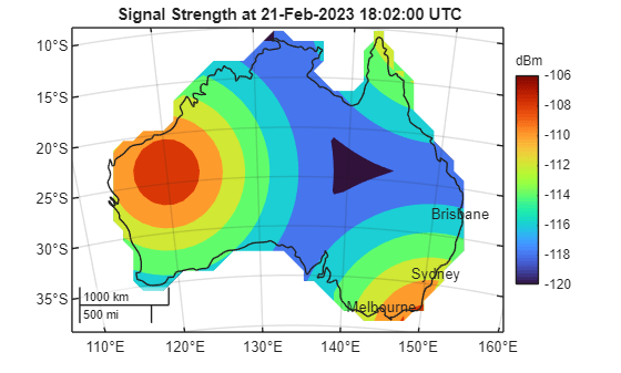
다른 관심 시간을 지정하고 커버리지를 계산하고 시각화합니다.
secondTOI = startTime + minutes(2); % 2 minutes after the start of the scenario
maxsigstrength = satcoverage(gridpts,sc,secondTOI,inregion,halfBeamWidth);

GT2 = contourDataGrid(gridlat,gridlon,maxsigstrength,levels,proj);
GT2 = sortrows(GT2,"Power (dBm)");

figure
newmap(proj)
hold on

colormap turbo
clim([minpowerlevel maxpowerlevel])
geoplot(GT2,ColorVariable="Power (dBm)",EdgeColor="none")
geoplot(australia,FaceColor="none")

cBar = colorbar;
title(cBar,"dBm");
title("Signal Strength at " + string(secondTOI) + " UTC")

text(sydney.Latitude,sydney.Longitude,"Sydney",HorizontalAlignment="center")
text(melbourne.Latitude,melbourne.Longitude,"Melbourne",HorizontalAlignment="center")
text(brisbane.Latitude,brisbane.Longitude,"Brisbane",HorizontalAlignment="center")
도시의 커버리지 수준 계산하기
호주 내 3개 도시의 커버리지 수준을 계산하고 표시합니다.
covlevels1 = [coveragelevel(sydney,GT); coveragelevel(melbourne,GT); coveragelevel(brisbane,GT)];
covlevels2 = [coveragelevel(sydney,GT2); coveragelevel(melbourne,GT2); coveragelevel(brisbane,GT2)];

covlevels = table(covlevels1,covlevels2, ...
    RowNames=["Sydney" "Melbourne" "Brisbane"], ...
    VariableNames=["Signal Strength at T1 (dBm)" "Signal Strength T2 (dBm)"])
covlevels=3×2 table
                 Signal Strength at T1 (dBm)    Signal Strength T2 (dBm)
                 ___________________________    ________________________

    Sydney                  -108                          -112
    Melbourne               -112                          -110
    Brisbane                -112                          -116
헬퍼 함수
satcoverage 헬퍼 함수는 커버리지 데이터를 반환합니다. 이 함수는 각 위성에 대해 시야 모양을 계산하고 위성 시야 내의 각 지상국 수신기에 대한 신호 강도를 계산합니다. 커버리지 데이터는 위성으로부터 수신되는 최대 신호 강도입니다.
function coveragedata = satcoverage(gridpts,sc,timeIn,inregion,halfBeamWidth)

    % Get satellites and ground station receivers
    sats = sc.Satellites;
    rxs = [sc.GroundStations.Receivers];

    % Get field-of-view shapes for all satellites
    fovs = satfov(sats,timeIn,halfBeamWidth);

    % Initialize coverage data
    coveragedata = NaN(size(gridpts));

    for satind = 1:numel(sats)
        fov = fovs(satind);

        % Find grid and rx locations which are within the satellite field-of-view
        gridInFOV = isinterior(fov,gridpts);
        rxInFOV = gridInFOV(inregion);

        % Compute sigstrength at grid locations using temporary link objects
        gridsigstrength = NaN(size(gridpts));
        if any(rxInFOV)
            tx = sats(satind).Transmitters;
            lnks = link(tx,rxs(rxInFOV));
            rxsigstrength = sigstrength(lnks,timeIn)+30; % Convert from dBW to dBm
            gridsigstrength(inregion & gridInFOV) = rxsigstrength;
            delete(lnks)
        end

        % Update coverage data with maximum signal strength found
        coveragedata = max(gridsigstrength,coveragedata);
    end
end
satfov 헬퍼 함수는 천저 지향과 구형 지구 모델을 가정하여 각 위성의 시야를 나타내는 geopolyshape 객체의 배열을 반환합니다.
function fovs = satfov(sats,timeIn,halfViewAngle)

    % Compute the latitude, longitude, and altitude of all satellites at the input time
    satstates = states(sats,timeIn,CoordinateFrame="geographic");

    fovs = createArray([1 numel(sats)],"geopolyshape");
    for satind = 1:numel(sats)
        lla = satstates(:,1,satind);

        % Find the Earth central angle using the beam view angle
        if isreal(acosd(sind(halfViewAngle)*(lla(3)+earthRadius)/earthRadius))
            % Case when Earth FOV is bigger than antenna FOV
            earthCentralAngle = 90-acosd(sind(halfViewAngle)*(lla(3)+earthRadius)/earthRadius)-halfViewAngle;
        else
            % Case when antenna FOV is bigger than Earth FOV
            earthCentralAngle = 90-halfViewAngle;
        end

        % Create a circular geopolyshape centered at the position of the satellite
        % with a buffer of width equaling the Earth central angle
        fovs(satind) = aoicircle(lla(1),lla(2),earthCentralAngle);
    end
end
contourDataGrid 헬퍼 함수는 데이터 그리드의 등고선을 그리고 결과를 지리공간 테이블로 반환합니다. 테이블의 각 행은 전력 수준에 해당하며 등고선 모양, 등고선 모양의 면적(제곱킬로미터), 해당 수준에 대한 최소 전력, 해당 수준에 대한 전력 범위를 포함합니다.
function GT = contourDataGrid(latd,lond,data,levels,proj)

    % Pad each side of the grid to ensure no contours extend past the grid bounds
    lond = [2*lond(1,:)-lond(2,:); lond; 2*lond(end,:)-lond(end-1,:)];
    lond = [2*lond(:,1)-lond(:,2) lond 2*lond(:,end)-lond(:,end-1)];
    latd = [2*latd(1,:)-latd(2,:); latd; 2*latd(end,:)-latd(end-1,:)];
    latd = [2*latd(:,1)-latd(:,2) latd 2*latd(:,end)-latd(:,end-1)];
    data = [ones(size(data,1)+2,1)*NaN [ones(1,size(data,2))*NaN; data; ones(1,size(data,2))*NaN] ones(size(data,1)+2,1)*NaN];

    % Replace NaN values in power grid with a large negative number
    data(isnan(data)) = min(levels) - 1000;

    % Project the coordinates using an equal-area projection
    [xd,yd] = projfwd(proj,latd,lond);

    % Contour the projected data
    fig = figure("Visible","off");
    obj = onCleanup(@()close(fig));
    c = contourf(xd,yd,data,LevelList=levels);

    % Initialize variables
    x = c(1,:);
    y = c(2,:);
    n = length(y);
    k = 1;
    index = 1;
    levels = zeros(n,1);
    latc = cell(n,1);
    lonc = cell(n,1);

    % Process the coordinates of the projected contours
    while k < n
        level = x(k);
        numVertices = y(k);
        yk = y(k+1:k+numVertices);
        xk = x(k+1:k+numVertices);
        k = k + numVertices + 1;

        [first,last] = findNanDelimitedParts(xk);
        jindex = 0;
        jy = {};
        jx = {};

        for j = 1:numel(first)
            % Process the j-th part of the k-th level
            s = first(j);
            e = last(j);
            cx = xk(s:e);
            cy = yk(s:e);
            if cx(end) ~= cx(1) && cy(end) ~= cy(1)
                cy(end+1) = cy(1); %#ok<*AGROW>
                cx(end+1) = cx(1);
            end

            if j == 1 && ~ispolycw(cx,cy)
                % First region must always be clockwise
                [cx,cy] = poly2cw(cx,cy);
            end

            % Filter regions made of collinear points or fewer than 3 points
            if ~(length(cx) < 4 || all(diff(cx) == 0) || all(diff(cy) == 0))
                jindex = jindex + 1;
                jy{jindex,1} = cy(:)';
                jx{jindex,1} = cx(:)';
            end
        end

        % Unproject the coordinates of the processed contours
        [jx,jy] = polyjoin(jx,jy);
        if length(jy) > 2 && length(jx) > 2
            [jlat,jlon] = projinv(proj,jx,jy);
            latc{index,1} = jlat(:)';
            lonc{index,1} = jlon(:)';
            levels(index,1) = level;
            index = index + 1;
        end
    end

    % Create contour shapes from the unprojected coordinates. Include the
    % contour shapes, the areas of the shapes, and the power levels in a
    % geospatial table.
    latc = latc(1:index-1);
    lonc = lonc(1:index-1);
    Shape = geopolyshape(latc,lonc);

    Area = area(Shape);

    levels = levels(1:index-1);
    Levels = levels;

    allPartsGT = table(Shape,Area,Levels);

    % Condense the geospatial table into a new geospatial table with one
    % row per power level.
    GT = table.empty;
    levels = unique(allPartsGT.Levels);
    for k = 1:length(levels)
        gtLevel = allPartsGT(allPartsGT.Levels == levels(k),:);
        tLevel = geotable2table(gtLevel,["Latitude","Longitude"]);
        [lon,lat] = polyjoin(tLevel.Longitude,tLevel.Latitude);
        Shape = geopolyshape(lat,lon);
        Levels = levels(k);
        Area = area(Shape);
        GT(end+1,:) = table(Shape,Area,Levels);
    end

    maxLevelDiff = max(abs(diff(GT.Levels)));
    LevelRange = [GT.Levels GT.Levels + maxLevelDiff];
    GT.LevelRange = LevelRange;

    % Clean up the geospatial table
    GT.Area = GT.Area/1e6;
    GT.Properties.VariableNames = ...
        ["Shape","Area (sq km)","Power (dBm)","Power Range (dBm)"];
end
coveragelevel 함수는 geopointshape 객체의 커버리지 수준을 반환합니다.
function powerLevels = coveragelevel(point,GT)

    % Determine whether points are within coverage
    inContour = false(length(GT.Shape),1);
    for k = 1:length(GT.Shape)
        inContour(k) = isinterior(GT.Shape(k),point);
    end

    % Find the highest coverage level containing the point
    powerLevels = max(GT.("Power (dBm)")(inContour));

    % Return -inf if the point is not contained within any coverage level
    if isempty(powerLevels)
        powerLevels = -inf;
    end
end
findNanDelimitedParts 헬퍼 함수는 배열 x의 NaN으로 구분된 각 부분에서 그 첫 번째 요소와 마지막 요소의 인덱스를 찾습니다.
function [first,last] = findNanDelimitedParts(x)

    % Find indices of the first and last elements of each part in x.
    % x can contain runs of multiple NaNs, and x can start or end with
    % one or more NaNs.

    n = isnan(x(:));

    firstOrPrecededByNaN = [true; n(1:end-1)];
    first = find(~n & firstOrPrecededByNaN);

    lastOrFollowedByNaN = [n(2:end); true];
    last = find(~n & lastOrFollowedByNaN);
end
참고 문헌
[1] Attachment EngineeringStatement SAT-MOD-20131227-00148. https://fcc.report/IBFS/SAT-MOD-20131227-00148/1031348. Accessed 17 Jan. 2023.
참고 항목
aoicircle (Mapping Toolbox)
도움말 항목
- Read Quantitative Data from WMS Server (Mapping Toolbox)