Compare DDPG Agent to LQR Controller
This example shows how to train a deep deterministic policy gradient (DDPG) agent to control a second-order linear dynamic system modeled in MATLAB®. The example also compares a DDPG agent with a custom quadratic approximation model to an LQR controller.
For more information on DDPG agents, see Deep Deterministic Policy Gradient (DDPG) Agent. For an example showing how to train a DDPG agent in a Simulink® environment, see Train Default DDPG Agent to Swing Up and Balance Continuous Pendulum and Control Water Level in a Tank Using a DDPG Agent.
Fix Random Number Stream for Reproducibility
The example code might involve computation of random numbers at several stages. Fixing the random number stream at the beginning of some sections in the example code preserves the random number sequence in the section every time you run it, which increases the likelihood of reproducing the results. For more information, see Results Reproducibility.
Fix the random number stream with seed 0 and random number algorithm Mersenne Twister. For more information on controlling the seed used for random number generation, see rng.
previousRngState = rng(0,"twister");The output previousRngState is a structure that contains information about the previous state of the stream. You will restore the state at the end of the example.
Continuous Action Space Double-Integrator MATLAB Environment
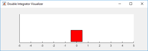
The reinforcement learning environment for this example is a second-order double-integrator system with a gain. The training goal is to control the position of a mass in the second-order system by applying a force input.
For this environment:
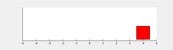
The mass starts at an initial position of either –4 or 4 m.
The observations from the environment are the position and velocity of the mass.
The episode terminates if the mass moves more than 5 m from the original position or if .
The reward , provided at every time step, is a discretization of :
Here:
is the state vector of the mass.
is the force applied to the mass.
is the matrix of weight on the state deviation from zero; .
is the weight on the control effort; .
For more information on this model, see Use Predefined Control System Environments.
For this example the environment is a linear dynamic system, the environment state is observed directly, and the reward is a quadratic function of the observation and action. Therefore the problem of finding the sequence of actions that minimizes the cumulative long-term reward is a discrete-time linear-quadratic optimal control problem, for which the optimal action is known to be a linear function of the system states. This problem can also be solved using Linear-Quadratic Regulator (LQR) design, and in the last part of the example you can compare the agent to an LQR controller.
Create Environment Object
Create a predefined environment object for the continuous action space double-integrator system.
env = rlPredefinedEnv("DoubleIntegrator-Continuous")env =
DoubleIntegratorContinuousAction with properties:
Gain: 1
Ts: 0.1000
MaxDistance: 5
GoalThreshold: 0.0100
Q: [2×2 double]
R: 0.0100
MaxForce: Inf
State: [2×1 double]
The agent can apply force values from -Inf to Inf to the mass. The sample time is stored in env.Ts, while the continuous time cost function matrices are stored in env.Q and env.R respectively.
Obtain the observation and action specifications from the environment.
obsInfo = getObservationInfo(env)
obsInfo =
  rlNumericSpec with properties:

     LowerLimit: -Inf
     UpperLimit: Inf
           Name: "states"
    Description: "x, dx"
      Dimension: [2 1]
       DataType: "double"
actInfo = getActionInfo(env)
actInfo =
  rlNumericSpec with properties:

     LowerLimit: -Inf
     UpperLimit: Inf
           Name: "force"
    Description: [0×0 string]
      Dimension: [1 1]
       DataType: "double"
Reset the environment and get its initial state.
x0 = reset(env)
x0 = 2×1

     4
     0
Create a DDPG Agent
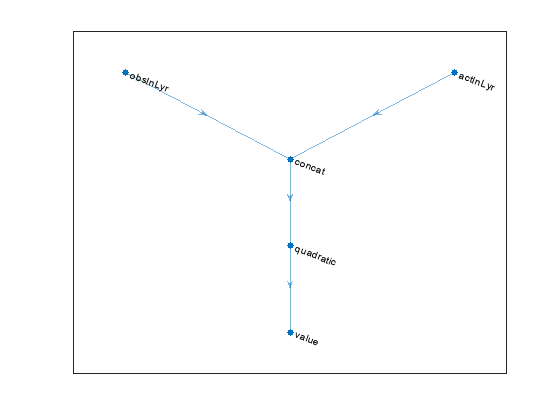
A DDPG agent approximates the discounted cumulative long-term reward using a Q-value function critic. A Q-value function critic must accept an observation and an action as inputs and return a scalar (the estimated discounted cumulative long-term reward) as output. To approximate the Q-value function within the critic, use a neural network. Because the value function of the optimal policy is known to be quadratic, use a network with a quadratic layer (which outputs a vector of quadratic monomials, as described in quadraticLayer) and a fully connected layer (which provides a linear combination of its inputs).
Define each network path as an array of layer objects, getting the dimension of the observation and action spaces from the environment specification objects. Assign names to the network input layers, so you can connect them to the output path and later explicitly associate them with the appropriate environment channel. Because there is no need for a bias term, set the bias term to zero (Bias=0) and prevent it from changing (BiasLearnRateFactor=0).
For more information on creating value function approximators, see Create Actors, Critics, and Policy Objects.
% Observation and action paths
obsPath = featureInputLayer(obsInfo.Dimension(1),Name="obsInLyr");
actPath = featureInputLayer(actInfo.Dimension(1),Name="actInLyr");

% Common path
commonPath = [
    concatenationLayer(1,2,Name="concat")
    quadraticLayer
    fullyConnectedLayer(1,Name="value", ...
        BiasLearnRateFactor=0,Bias=0)
    ];
Create dlnetwork object and add layers.
criticNet = dlnetwork;
criticNet = addLayers(criticNet,obsPath);
criticNet = addLayers(criticNet,actPath);
criticNet = addLayers(criticNet,commonPath);
Connect layers.
criticNet = connectLayers(criticNet,"obsInLyr","concat/in1");
criticNet = connectLayers(criticNet,"actInLyr","concat/in2");
View the critic network configuration.
plot(criticNet)
Initialize network and display the number of weights.
criticNet = initialize(criticNet);
summary(criticNet)
   Initialized: true

   Number of learnables: 7

   Inputs:
      1   'obsInLyr'   2 features
      2   'actInLyr'   1 features
Create the critic object using criticNet, the environment observation and action specifications, and the names of the network input layers to be connected with the environment observation and action channels, respectively. For more information, see rlQValueFunction.
critic = rlQValueFunction(criticNet, ...
    obsInfo,actInfo, ...
    ObservationInputNames="obsInLyr", ...
    ActionInputNames="actInLyr");
Check the critic with a random observation and action input.
getValue(critic,{rand(obsInfo.Dimension)},{rand(actInfo.Dimension)})ans = single
-0.3762
DDPG agents use a parameterized continuous deterministic policy, which is learned by a continuous deterministic actor. This actor must accept an observation as input and return an action as output. To approximate the policy function within the actor, use a neural network. Because for this example the optimal policy is known to be linear in the state, use a shallow network with a fully connected layer to provide a linear combination of the two elements of the observation (position and velocity of the mass).
Define the network as an array of layer objects, and get the dimension of the observation and action spaces from the environment specification objects. Because there is no need for a bias term, as done for the critic, set the bias term to zero (Bias=0) and prevent it from changing (BiasLearnRateFactor=0). For more information on actors, see Create Actors, Critics, and Policy Objects.
actorNet = [
    featureInputLayer(obsInfo.Dimension(1))
    fullyConnectedLayer(actInfo.Dimension(1), ...
        BiasLearnRateFactor=0,Bias=0)
    ];
Convert to dlnetwork, initialize network, and display the number of weights.
actorNet = dlnetwork(actorNet);
actorNet = initialize(actorNet);
summary(actorNet)
   Initialized: true

   Number of learnables: 3

   Inputs:
      1   'input'   2 features
Create the actor using actorNet and the observation and action specifications. For more information, see rlContinuousDeterministicActor.
actor = rlContinuousDeterministicActor(actorNet,obsInfo,actInfo);
Check the actor with a random observation input.
getAction(actor,{rand(obsInfo.Dimension)})ans = 1×1 cell array
{[-0.2809]}
Create the DDPG agent using the actor and critic. For more information, see rlDDPGAgent.
agent = rlDDPGAgent(actor,critic);
Specify options for the agent, including training options for the critic, using dot notation. Alternatively, you can use rlDDPGAgentOptions, and rlOptimizerOptions objects before creating the agent.
Set the agent sample time. This ensures that the time interval between consecutive elements in the returned experience is Ts. It also ensures that if you use the agent in an RL Agent block, the block executes at intervals of Ts seconds.
agent.AgentOptions.SampleTime = env.Ts;
Specify a capacity of 1e6 for the experience buffer to store a diverse set of experiences. Also specify a mini-batch size of 32 for learning. Smaller mini-batches are computationally efficient though they might introduce variance in training. Contrarily, larger batch sizes can make the training stable but require higher memory.
agent.AgentOptions.ExperienceBufferLength = 1e5;
agent.AgentOptions.MiniBatchSize = 32;
Specify a decay rate of 1e-5 for the noise standard deviation to gradually decay during training. This promotes exploration toward the beginning when the agent does not have a good policy, and exploitation toward the end when the agent has learned the optimal policy.
agent.AgentOptions.NoiseOptions.StandardDeviationDecayRate = 1e-5;
Specify a learning rate of 1e-3 for the agent actor and critic optimizer algorithms. A large learning rate causes drastic updates which might lead to divergent behaviors, while a low value might require many updates before reaching the optimal point. Also specify a gradient threshold value of 1.0 to clip the computed gradients to enhance the stability of the learning algorithm.
agent.AgentOptions.ActorOptimizerOptions.LearnRate = 1e-3;
agent.AgentOptions.ActorOptimizerOptions.GradientThreshold = 1;
agent.AgentOptions.CriticOptimizerOptions.LearnRate = 5e-3;
agent.AgentOptions.CriticOptimizerOptions.GradientThreshold = 1;
Initialize Agent Parameters
Extract Parameters from Agent
Extract the actor and critic parameters from the agent.
par = getLearnableParameters(agent);
Actor Parameters
The policy implemented by the actor is , where the feedback gains and are the two weights of the actor network. It can be shown that the closed loop system is stable if these gains are negative, therefore, initializing them to negative values can speed up convergence.
Set the gains and , to -1.
K = [-1 -1];
Set the actor parameters to .
par.Actor{1} = single(K);Critic Parameters
Because the critic uses quadraticLayer followed by a fullyConnectedLayer, the Q-value function has the following structure:
where are the weights of the fully connected layer. Alternatively, in matrix form:
.
For a fixed policy , the cumulative long-term reward (that is, the value of the policy) becomes:
.
Because the rewards are always negative, to properly approximate the cumulative reward, both matrices and must be negative definite. Therefore, to speed up convergence, initialize the critic network weights so that the matrix is negative definite. Set the critic parameter vector to [-1.1, -0.1, -1.1, -0.1, -0.1, -1.1].
W = [-1, -0.1, -1, -0.1, -0.1, -1.1];
Build the matrix .
WQ = [W(1) W(2)/2 W(4)/2; W(2)/2 W(3) W(5)/2; W(4)/2 W(5)/2 W(6)];
Build the matrix .
P = [eye(2) K']*WQ*[eye(2);K];
Check that both matrices have negative eigenvalues:
eig(WQ)
ans = 3×1

   -1.1500
   -1.0000
   -0.9500
eig(P)
ans = 2×1

   -3.0500
   -0.9500
Set the critic parameters to the vector .
par.Critic{1} = single(W);Set Parameters back in the Agent and Check Agent
Set the parameters of both actor and critic in the agent.
setLearnableParameters(agent,par);
Check the agent with a random observation input.
getAction(agent,{rand(obsInfo.Dimension)})ans = 1×1 cell array
{[-0.9422]}
Train Agent
To train the agent, first specify the training options. For this example, use the following options.
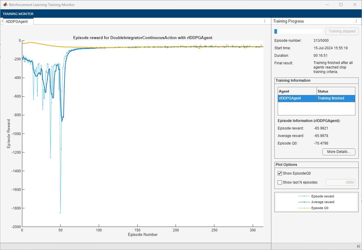
Run a maximum of
5000episodes in the training session, with each episode lasting a maximum of200time steps.Display the training progress in the Reinforcement Learning Training Monitor dialog box (set the
Plotsoption) and disable the command line display (Verboseoption).Stop the training when the agent receives a moving average cumulative reward (over the default value of 5 episodes) greater than
–66. At this point, the agent can control the position of the mass using minimal control effort.
For more information on training options, see rlTrainingOptions.
trainOpts = rlTrainingOptions( ...
    MaxEpisodes=5000, ...
    MaxStepsPerEpisode=200, ...
    Verbose=false, ...
    Plots="training-progress", ...
    StopTrainingCriteria="AverageReward", ...
    StopTrainingValue=-66);
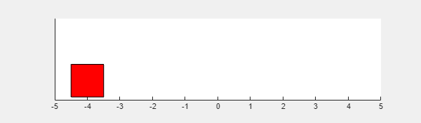
You can visualize the double-integrator environment by using the plot function during training or simulation.
plot(env)
Train the agent using train. Training this agent is a computationally intensive process that takes several hours to complete. To save time while running this example, load a pretrained agent by setting doTraining to false. To train the agent yourself, set doTraining to true.
doTraining =false; if doTraining % Train the agent. trainingStats = train(agent,env,trainOpts); else % Load the pretrained agent for the example. load("DoubleIntegDDPG.mat","agent"); end
Simulate Trained Agent
To validate the performance of the trained agent, simulate it within the double-integrator environment. For more information on agent simulation, see rlSimulationOptions and sim.
simOptions = rlSimulationOptions(MaxSteps=500);
experience = sim(env,agent,simOptions);

totalReward = sum(experience.Reward)
totalReward =
-65.9806
Solve LQR Problem
The function lqrd (Control System Toolbox) solves a discretized LQR problem, like the one presented in this example. This function calculates the optimal discrete-time gain matrix Klqr, together with the solution of the Riccati equation Plqr. When Klqr is connected via negative state feedback to the plant input (force), the discrete-time equivalent of the cost function specified by env.Q and env.R is minimized going forward. Furthermore, the cumulative cost from initial time to infinity, starting from an initial state x0, is equal to x0'*Plqr*x0.
Use lqrd to solve the discretized LQR problem.
[Klqr,Plqr] = lqrd([0 1;0 0],[0;env.Gain],env.Q,env.R,env.Ts);
Here, [0 1;0 0] and [0;env.Gain] are the continuous-time transition and input gain matrices, respectively, of the double-integrator system.
If Control System Toolbox™ is not installed, use the solution for the default example values.
Klqr = [17.8756 8.2283];
Plqr = [4.1031 0.3376; 0.3376 0.1351];
If the actor policy successfully approximates the optimal policy, then the resulting must be close to (the minus sign is due to the fact that is calculated assuming a negative feedback connection).
If the critic learns a good approximation of the optimal value function, then the resulting , as defined before, must be close to (the minus sign is due to the fact that the reward is defined as the negative of the cost).
Compare DDPG Agent to Optimal Controller
Extract the parameters (weighs) of the actor and critic within the agent.
par = getLearnableParameters(agent);
Compare Actor Parameters to LQR Gains
Obtain and display the actor weights.
K = par.Actor{1}K = 1×2 single row vector
-15.4663 -7.2746
Check whether the gains are close to the ones of the optimal solution -Klqr:
-Klqr
ans = 1×2

  -17.8756   -8.2283
The two matrices K and -Klqr are very similar.
Compare Critic Value Functions
Obtain and display the critic weights.
W = par.Critic{1}W = 1×6 single row vector
-5.0017 -1.5513 -0.3424 -0.1116 -0.0506 -0.0047
Recreate the matrices and .
WQ = [W(1) W(2)/2 W(4)/2; W(2)/2 W(3) W(5)/2; W(4)/2 W(5)/2 W(6)];
P = [eye(2) K']*WQ*[eye(2);K] ...
P = 2×2 single matrix
-4.4050 -0.5099
-0.5099 -0.2244
Check whether is close to the solution of the Riccati equation -Plqr.
-Plqr
ans = 2×2

   -4.1031   -0.3376
   -0.3376   -0.1351
The two matrices P and -Plqr are very similar.
Get the environment initial state.
x0=reset(env);
The value function is the estimate of future cumulative long-term reward when using the policy enacted by the actor. Calculate the value function at the initial state, according to the critic weights. This is the same value displayed in the training window as Episode Q0.
q0 = x0'*P*x0
q0 = single

-70.4798
Calculate the value of the initial state, following the true optimal policy enacted by the LQR controller.
-x0'*Plqr*x0
ans =
-65.6494
The two approximations of the value of the initial state are close to each other, and are also close to the total cumulative reward obtained in the validation simulation, totalReward, suggesting that the critic learns a good approximation of the value function for the policy enacted by the actor.
Restore the random number stream using the information stored in previousRngState.
rng(previousRngState);
See Also
Apps
Functions
Objects
Topics
- Train PG Agent with Custom Actor and Baseline Networks to Control Discrete Double Integrator
- Train Default DDPG Agent to Swing Up and Balance Continuous Pendulum
- Tune Single PI Controller Gains For Multiple Operating Points Using Reinforcement Learning
- Create and Train Custom LQR Agent
- Use Predefined Control System Environments
- Deep Deterministic Policy Gradient (DDPG) Agent
- Create Actors, Critics, and Policy Objects
- Train Reinforcement Learning Agents