Train Reinforcement Learning Agents to Control Quanser QUBE Pendulum
This example trains reinforcement learning (RL) agents to swing up and control a Quanser QUBE™-Servo 2 inverted pendulum system.
Fix Random Number Stream for Reproducibility
The example code might involve computation of random numbers at various stages. Fixing the random number stream at the beginning of various sections in the example code preserves the random number sequence in the section every time you run it, and increases the likelihood of reproducing the results. For more information, see Results Reproducibility.
Fix the random number stream with seed 0 and random number algorithm Mersenne twister. For more information on controlling the seed used for random number generation, see rng.
previousRngState = rng(0,"twister");The output previousRngState is a structure that contains information about the previous state of the stream. You will restore the state at the end of the example.
Inverted Pendulum Model
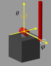
The Quanser QUBE-Servo 2 pendulum system is a rotational inverted pendulum with two degrees of freedom. It is non-linear, underactuated, non-minimum phase, and it is modeled in Simulink using Simscape™ Electrical™ and Simscape Multibody™. For a detailed description of the dynamics, see [1].
The pendulum is attached to the motor arm through a free revolute joint. The arm is actuated by a DC motor. The environment has the following properties:
The angles and angular velocities of the motor arm (,) and pendulum (,) are measurable.
The motor is constrained to and .
The pendulum is upright when .
The motor input is constrained to .
The agent action is scaled to the motor voltage in the environment.
Open the Simulink model.
mdl = "rlQubeServo";
open_system(mdl)
Define the limit for (radians), (radians/second), voltage limit (volts), as well as the agent's sample time (seconds).
theta_limit = 5*pi/8;
dtheta_limit = 30;
volt_limit = 12;
Ts = 0.005;
Define the initial conditions for ,,,.
theta0 = 0;
phi0 = 0;
dtheta0 = 0;
dphi0 = 0;

Create Environment Object
For this environment:
The pendulum system modeled in Simscape Multibody.
The observation is the vector . Using the sine and cosine of the measured angles can facilitate training by representing the otherwise discontinuous angular measurements by a continuous two-dimensional parametrization.
The action is the normalized input voltage command to the servo motor.
The reward signal is defined as follows:
.
The above reward function penalizes six different terms:
Deviations from the forward position of the motor arm ().
Deviations for the inverted position of the pendulum ().
The angular speed of the motor arm .
The angular speed of the pendulum .
The control action .
Changes to the control action .
The agent is rewarded while the system constraints are satisfied (that is ).
Create the input and output specifications for the agent. Set the action upper and lower limits to constrain the actions selected by the agent.
obsInfo = rlNumericSpec([7 1]);
actInfo = rlNumericSpec([1 1],UpperLimit=1,LowerLimit=-1);
Create the environment object. Specify a reset function, defined at the end of the example, that sets random initial conditions.
agentBlk = mdl + "/RL Agent";
env = rlSimulinkEnv(mdl,agentBlk,obsInfo,actInfo);
env.ResetFcn = @localResetFcn;
Create TD3 Agent
The agent used in this example is a twin-delayed deep deterministic policy gradient (TD3) agent. TD3 agents use two parametrized Q-value function approximators to estimate the value (that is the expected cumulative long-term reward) of the policy.
To model the parametrized Q-value function within both critics, use a neural network with two inputs (the observation and action) and one output (the value of the policy when taking a given action from the state corresponding to a given observation). For more information on TD3 agents, see Twin-Delayed Deep Deterministic (TD3) Policy Gradient Agent.
Create an agent initialization object to initialize the critic network with the hidden layer size 64.
initOpts = rlAgentInitializationOptions(NumHiddenUnit=64);
Specify the agent options for training using rlTD3AgentOptions and rlOptimizerOptions objects. For this training:
Use an experience buffer with capacity 1e6 to collect experiences. A larger capacity maintains a diverse set of experiences in the buffer.
Use mini-batches of 1024 experiences. Smaller mini-batches are computationally efficient but may introduce variance in training. By contrast, larger batch sizes can make the training stable but require higher memory.
Use a total of 10 learning epochs to train the agent networks.
Use the stochastic gradient descent with momentum (SGDM) algorithm to update the actor and critic neural networks.
Specify the learning rate of 2e-3 for the actor and 5e-3 for the critics, and a gradient threshold of 1 for both the actor and the critics.
Specify the initial standard deviation value of 0.5 for the gaussian exploration model. The standard deviation decays at the rate of 1e-6 which facilitates exploration towards the beginning and exploitation towards the end of training.
agentOpts = rlTD3AgentOptions( ...
    SampleTime=Ts, ...
    ExperienceBufferLength=1e6, ...
    MiniBatchSize=1024, ...
    NumEpoch=10);

agentOpts.ActorOptimizerOptions.Algorithm = "sgdm";
agentOpts.ActorOptimizerOptions.LearnRate = 2e-3;
agentOpts.ActorOptimizerOptions.GradientThreshold = 1;
for i = 1:2
    agentOpts.CriticOptimizerOptions(i).Algorithm = "sgdm";
    agentOpts.CriticOptimizerOptions(i).LearnRate = 5e-3;
    agentOpts.CriticOptimizerOptions(i).GradientThreshold = 1;
end

agentOpts.ExplorationModel.StandardDeviation = 0.5;
agentOpts.ExplorationModel.StandardDeviationDecayRate = 1e-6;
Create the TD3 agent using the observation and action input specifications, initialization options and agent options. When you create the agent, the initial parameters of the critic network are initialized with random values. Fix the random number stream so that the agent is always initialized with the same parameter values.
rng(0,"twister");
agent = rlTD3Agent(obsInfo,actInfo,initOpts,agentOpts);
Train Agent
To train the agent, first specify the training options. For this example, use the following options:
Run the training for 2000 episodes, with each episode lasting at most
maxStepstime steps.Specify an averaging window of 10 for the episode rewards.
Tf = 5;
maxSteps = ceil(Tf/Ts);
trainOpts = rlTrainingOptions(...
    MaxEpisodes=2000, ...
    MaxStepsPerEpisode=maxSteps, ...
    ScoreAveragingWindowLength=10, ...
    StopTrainingCriteria="none");
To train the agent in parallel, specify the following training options. Training in parallel requires Parallel Computing Toolbox™ software. If you do not have Parallel Computing Toolbox™ software installed, set UseParallel to false.
Set the
UseParalleloption totrue.Train the agent using asynchronous parallel workers.
trainOpts.UseParallel =true; trainOpts.ParallelizationOptions.Mode =
"async";
For more information see rlTrainingOptions.
In parallel training, workers simulate the agent's policy with the environment and store experiences in the replay memory. When workers operate asynchronously the order of stored experiences may not be deterministic and can ultimately make the training results different. To maximize the reproducibility likelihood:
Initialize the parallel pool with the same number of parallel workers every time you run the code. For information on specifying the pool size see Discover Clusters and Use Cluster Profiles (Parallel Computing Toolbox).
Use synchronous parallel training by setting
trainOpts.ParallelizationOptions.Modeto"sync".Assign a random seed to each parallel worker using
trainOpts.ParallelizationOptions.WorkerRandomSeeds. The default value of -1 assigns a unique random seed to each parallel worker.
Create an evaluator object to evaluate the performance of the greedy policy every 20 training episodes, averaging the cumulative reward of 5 simulations.
evl = rlEvaluator(EvaluationFrequency=20, NumEpisodes=5);
Fix the random stream for reproducibility.
rng(0,"twister");Train the agent using the train function. Training this agent is a computationally intensive process that takes several minutes to complete. To save time while running this example, load a pretrained agent by setting doTraining to false. To train the agent yourself, set doTraining to true.
doTraining =false; if doTraining % Train the agent. trainingStats = train(agent,env,trainOpts, ... Evaluator=evl); else % Load the pretrained agent for the example. load("rlQubeServoAgents.mat","agent") end
A snapshot of the training progress is shown below. You may expect different results due to randomness in training.

Simulate Agent
Fix the random stream for reproducibility.
rng(0,"twister");Define simulation options.
simOpts = rlSimulationOptions(MaxSteps=maxSteps);
Simulate the trained agent.
experience = sim(agent,env,simOpts);
View the performance of the agents in the Simulation Data Inspector. To open the Simulation Data Inspector, in the Simulink model window, on the Simulation tab, in the Review Results gallery, click Data Inspector.
In the plots:
The measured values for (
theta_wrapped) and (phi_wrapped) are stabilized at approximately0radians. The pendulum is stabilized at the upright equilibrium position.The
actsignal shows the actions of the agent.The control input is shown by the
voltsignal.

Restore the random number stream using the information stored in previousRngState.
rng(previousRngState);
Local Functions
The function localResetFcn resets the initial angles to a random number and the initial speeds to 0.
function in = localResetFcn(in)
theta0 = -pi/4+rand*pi/2;
phi0 = pi-pi/4+rand*pi/2;
in = setVariable(in,"theta0",theta0);
in = setVariable(in,"phi0",phi0);
in = setVariable(in,"dtheta0",0);
in = setVariable(in,"dphi0",0);
end
See Also
Functions
train|sim|rlSimulinkEnv
Objects
Blocks
Topics
- Train Reinforcement Learning Agent Offline to Control Quanser QUBE Pendulum
- Train DQN Agent to Swing Up and Balance Pendulum
- Train DDPG Agent to Swing Up and Balance Pendulum
- Run SIL and PIL Verification for Reinforcement Learning
- Train Multiple Agents to Perform Collaborative Task
- Create Custom Simulink Environments
- Proximal Policy Optimization (PPO) Agent
- Soft Actor-Critic (SAC) Agent
- Train Reinforcement Learning Agents