이 번역 페이지는 최신 내용을 담고 있지 않습니다. 최신 내용을 영문으로 보려면 여기를 클릭하십시오.
3축 진동 데이터를 사용하여 산업 기계의 이상 감지하기
일반적으로 이상(anomalous) 동작에 대한 것보다 정상(nominal) 동작에 사용할 수 있는 데이터가 훨씬 더 많기 때문에 기계에서 이상을 감지하는 것은 종종 어려운 일일 수 있습니다. 2-클래스 모델 훈련의 경우, 이러한 데이터 불균형은 훈련된 모델에서 더 큰 클래스 쪽으로 편향된 결과를 낳을 수 있습니다.
정상 데이터와 이상 데이터를 모두 사용하여 모델을 훈련시키는 다른 접근 방식은 모델이 바깥쪽 데이터를 이상 데이터로 감지하는 충실도 수준이 될 때까지 정상 데이터만으로 모델을 훈련시키는 것입니다.
이 예제에서는 이러한 접근 방식을 통해 머신러닝과 딥러닝의 모델을 사용하여 산업 기계의 진동 데이터에서 이상을 감지하는 방법을 보여줍니다. 여기서는 기계 데이터가 유지관리 전에는 이상 데이터이고 유지관리 후에는 정상 데이터라고 간주합니다. 다음 그림에 표시된 대로, 이러한 구분을 통해 훈련에는 정상 데이터만 사용되고 테스트에는 혼합 데이터가 사용됩니다.

이 과정에는 다음 단계가 포함됩니다.
1) 진단 특징 디자이너 앱에서 축소된 데이터 세트를 사용하여 원시 진동 측정값에서 특징을 추출하고, 특징에 순위를 지정하고, 특징을 선택합니다. 그런 다음, 앱에서 생성된 코드를 사용하여 전체 데이터 세트에 대해 선택된 특징을 생성합니다.
2) 이 특징 데이터를 훈련 세트와 독립적인 테스트 세트로 분할합니다. 그런 다음, 훈련 세트에서 레이블이 'After'인 모든 특징을 추출하여 정상 데이터만 포함된 새 훈련 세트를 만듭니다.
3) 독립적인 테스트 세트는 그대로 유지합니다. 이 테스트 세트에는 'Before'(이상) 또는 'After'(정상) 레이블을 갖는 데이터가 혼합되어 들어 있습니다.
4) 훈련 세트를 사용하여 이상 감지에 대해 3개의 다른 모델(단일 클래스 SVM, 격리 포레스트, LSTM 신경망)을 훈련시킵니다.
5) 테스트 세트를 사용하여 각각의 훈련된 모델을 테스트해서, 각 신호가 이상 신호인지 또는 정상 신호인지를 모델이 얼마나 잘 식별하는지 평가하고 비교합니다.
데이터 세트를 다운로드하고 불러오기
레이블이 지정된 3축 진동 측정값을 포함하는 데이터 세트를 다운로드하고 압축을 푼 다음 불러옵니다.
url = 'https://ssd.mathworks.com/supportfiles/predmaint/anomalyDetection3axisVibration/v1/vibrationData.zip';
websave('vibrationData.zip',url);
unzip('vibrationData.zip');
load("MachineData.mat")
head(trainData,3)
          ch1                 ch2                 ch3           label
    ________________    ________________    ________________    ______

    {70000×1 double}    {70000×1 double}    {70000×1 double}    Before
    {70000×1 double}    {70000×1 double}    {70000×1 double}    Before
    {70000×1 double}    {70000×1 double}    {70000×1 double}    Before
각 축의 데이터는 개별 열에 저장됩니다. 유지관리 전에 수집된 데이터의 레이블은 Before이고, 이 데이터는 이상 데이터로 간주됩니다. 유지관리 후에 수집된 데이터의 레이블은 'After'이고, 이 데이터는 정상 데이터로 간주됩니다.
데이터를 더 잘 이해할 수 있도록 유지관리 전과 후의 데이터를 시각화합니다. 앙상블의 네 번째 멤버에 대한 진동 데이터를 플로팅하고 두 상태에 대해 플로팅된 데이터가 다르게 나타나는 것을 확인합니다.
ensMember = 4;
helperPlotVibrationData(trainData, ensMember)

진단 특징 디자이너 앱을 사용하여 특징 추출하기
원시 데이터는 상관 관계가 있고 잡음이 있을 수 있기 때문에 머신러닝 모델을 훈련시키는 데 원시 데이터를 사용하는 것은 효율적이지 않습니다. Diagnostic Feature Designer 앱을 사용하면 대화형 방식으로 데이터를 탐색 및 전처리하고 시간 영역과 주파수 영역의 특징을 추출한 다음 특징에 순위를 지정하여 결함이나 이상이 있는 시스템 진단에 가장 효과적인 특징을 결정할 수 있습니다. 그런 다음 프로그래밍 방식으로 데이터 세트에서 선택한 특징을 추출하는 함수를 내보낼 수 있습니다. 명령 프롬프트에 diagnosticFeatureDesigner를 입력하여 진단 특징 디자이너를 엽니다. 진단 특징 디자이너를 사용하는 방법에 대한 튜토리얼은 예측 정비 알고리즘을 위한 상태 지표 설계하기 항목을 참조하십시오.
새 세션 버튼을 클릭하고 소스로 trainData를 선택한 다음 label을 상태 변수로 설정합니다. label 변수는 해당하는 데이터에 대한 기계 상태를 식별합니다.

진단 특징 디자이너를 사용하여 특징을 반복하고 순위를 지정할 수 있습니다. 앱은 생성된 모든 특징에 대한 히스토그램 보기를 만들어 각 레이블의 분포를 시각화합니다. 예를 들어 다음 히스토그램은 ch1에서 추출한 다양한 특징의 분포를 보여줍니다. 이러한 히스토그램은 레이블 그룹 분리를 더 잘 설명하기 위해 이 예제에서 사용하는 데이터 세트보다 훨씬 큰 데이터 세트에서 도출됩니다. 현재는 더 작은 데이터 세트를 사용하고 있기 때문에 결과가 다르게 보일 수 있습니다.

각 채널에 대해 상위 4개의 순위 특징을 사용합니다.
ch1: 파고율, 첨도, RMS, 표준편차ch2: 평균, RMS, 왜도, 표준편차ch3: 파고율, SINAD, SNR, THD
진단 특징 디자이너 앱에서 특징을 생성하는 함수를 내보내고 이름 generateFeatures로 저장합니다. 이 함수는 명령줄에서 전체 데이터 세트의 각 채널에서 상위 4개의 관련 특징을 추출합니다.
trainFeatures = generateFeatures(trainData);
head(trainFeatures(:,1:6))
    label     ch1_stats/Col1_CrestFactor    ch1_stats/Col1_Kurtosis    ch1_stats/Col1_RMS    ch1_stats/Col1_Std    ch2_stats/Col1_Mean
    ______    __________________________    _______________________    __________________    __________________    ___________________

    Before              2.2811                      1.8087                   2.3074                2.3071               -0.032332
    Before              2.3276                      1.8379                   2.2613                 2.261                -0.03331
    Before              2.3276                      1.8626                   2.2613                2.2612               -0.012052
    Before              2.8781                      2.1986                   1.8288                1.8285               -0.005049
    Before              2.8911                        2.06                   1.8205                1.8203              -0.0018988
    Before              2.8979                      2.1204                   1.8163                1.8162              -0.0044174
    Before              2.9494                        1.92                   1.7846                1.7844              -0.0067284
    Before              2.5106                      1.6774                   1.7513                1.7511              -0.0089548
훈련 및 테스트를 위한 전체 데이터 세트 준비하기
지금까지 사용한 데이터 세트는 특징을 추출하고 선택하는 과정을 설명하기 위한 것으로 훨씬 더 큰 데이터 세트의 일부에 불과합니다. 사용 가능한 모든 데이터로 알고리즘을 훈련시키면 최상의 성과를 얻을 수 있습니다. 이를 위해, 앞에서 추출한 것과 동일한 12개의 특징을 17,642개 신호로 이루어진 더 큰 데이터 세트에서 불러옵니다.
load("FeatureEntire.mat")
head(featureAll(:,1:6))
label ch1_stats/Col1_CrestFactor ch1_stats/Col1_Kurtosis ch1_stats/Col1_RMS ch1_stats/Col1_Std ch2_stats/Col1_Mean
______ __________________________ _______________________ __________________ __________________ ___________________
Before 2.3683 1.927 2.2225 2.2225 -0.015149
Before 2.402 1.9206 2.1807 2.1803 -0.018269
Before 2.4157 1.9523 2.1789 2.1788 -0.0063652
Before 2.4595 1.8205 2.14 2.1401 0.0017307
Before 2.2502 1.8609 2.3391 2.339 -0.0081829
Before 2.4211 2.2479 2.1286 2.1285 0.011139
Before 3.3111 4.0304 1.5896 1.5896 -0.0080759
Before 2.2655 2.0656 2.3233 2.3233 -0.0049447
cvpartition을 사용하여 데이터를 훈련 세트와 독립적인 테스트 세트로 분할합니다. helperExtractLabeledData 헬퍼 함수를 사용하여 featureTrain 변수에서 레이블 'After'에 해당하는 모든 특징을 찾습니다.
rng(0) % set for reproducibility
idx = cvpartition(featureAll.label, 'holdout', 0.1);
featureTrain = featureAll(idx.training, :);
featureTest = featureAll(idx.test, :);
정상인 것으로 간주되는 유지관리 이후의 데이터에 대해서만 각 모델을 훈련합니다. featureTrain에서 이 데이터만 추출합니다.
trueAnomaliesTest = featureTest.label;
featureNormal = featureTrain(featureTrain.label=='After', :);
단일 클래스 SVM을 사용하여 이상 감지하기
서포트 벡터 머신은 강력한 분류기로, 여기서는 정상 데이터에 대해서만 훈련하도록 변형하여 사용합니다. 이 모델은 정상 데이터와 "거리가 먼" 이상을 식별하는 데 매우 효과적입니다. ocsvm 함수와 정상 상태 데이터를 사용하여 단일 클래스 SVM 모델을 훈련시킵니다.
rng(0) % For reproducibility
mdlOCSVM = ocsvm(featureNormal{:,2:13}, "ContaminationFraction", 0, "StandardizeData", true, "KernelScale", 4);
정상 데이터와 이상 데이터가 모두 포함된 테스트 데이터를 사용하여 훈련된 SVM 모델을 검증합니다.
featureTestNoLabels = featureTest(:, 2:end);
isanomalyOCSVM = isanomaly(mdlOCSVM, featureTestNoLabels.Variables, "ScoreThreshold", -0.4);
predOCSVM = categorical(isanomalyOCSVM, [1, 0], ["Anomaly", "Nominal"]);

trueAnomaliesTest = renamecats(trueAnomaliesTest,["After","Before"], ["Nominal","Anomaly"]);
figure;
confusionchart(trueAnomaliesTest, predOCSVM, Title="Anomaly Detection with One-class SVM", Normalization="row-normalized");

혼동행렬을 통해 단일 클래스 SVM이 참양성 식별 비율은 높고 오분류 비율은 매우 작아, 좋은 성능을 보이는 것을 알 수 있습니다.
격리 포레스트를 사용하여 이상 감지하기
격리 포레스트의 결정 트리는 각 관측값을 리프로 격리합니다. 한 샘플이 리프에 도달하기까지 거쳐야 하는 결정의 수는 해당 샘플을 다른 샘플로부터 격리하는 것이 얼마나 어려운지 나타내는 척도입니다. 특정 샘플에 대한 트리의 평균 깊이가 이상 점수로 사용되며 iforest에 의해 반환됩니다.
정상 데이터로만 격리 포레스트 모델을 훈련시킵니다.
[mdlIF,~,scoreTrainIF] = iforest(featureNormal{:,2:13},'ContaminationFraction',0, 'NumLearners', 200, "NumObservationsPerLearner", 512);테스트 데이터를 사용하여 훈련된 격리 포레스트 모델을 검증합니다. 혼동행렬 차트를 사용하여 이 모델의 성능을 시각화합니다.
[isanomalyIF,scoreTestIF] = isanomaly(mdlIF,featureTestNoLabels.Variables, 'ScoreThreshold', 0.535);
predIF = categorical(isanomalyIF, [1, 0], ["Anomaly", "Nominal"]);
figure;
confusionchart(trueAnomaliesTest,predIF,Title="Anomaly Detection with Isolation Forest",Normalization="row-normalized");

이 데이터에서 격리 포레스트는 단일 클래스 SVM만큼 성능이 좋지 않습니다. 추가적인 데이터 및 하이퍼파라미터 조정 활동을 통해 격리 포레스트 모델의 성능을 더욱 개선할 수 있습니다.
양방향 LSTM 신경망을 사용하여 이상 감지하기
BiLSTM(양방향 LSTM) 신경망은 과거 문맥과 미래 문맥을 모두 고려하여 시퀀스 데이터를 처리하도록 설계된 신경망의 한 유형입니다. BiLSTM 신경망은 시계열 데이터의 순차적 종속성을 이해하는 능력이 탁월합니다. 이러한 이유로, 정상 데이터 시퀀스만 사용하여 BiLSTM 신경망을 훈련시켜서 이 신경망이 예상 패턴을 따르지 않는 신호에서 이상 또는 편차를 효과적으로 식별할 수 있습니다.
먼저 유지관리 후의 데이터에서 특징을 추출합니다.
featuresAfter = helperExtractLabeledData(featureTrain, ...
   "After");
BiLSTM 신경망을 생성하고 훈련 옵션을 설정합니다.
featureDimension = 1;

% Define biLSTM network layers
layers = [ sequenceInputLayer(featureDimension)
   bilstmLayer(16)
   reluLayer
   bilstmLayer(32)
   reluLayer
   bilstmLayer(16)
   reluLayer
   fullyConnectedLayer(featureDimension)];

% Set Training Options
options = trainingOptions('adam', ...
   'Plots', 'training-progress', ...
   'Metrics', 'rmse', ...
   'MiniBatchSize', 500,...
   'MaxEpochs',200, ...
   'Verbose',false);
MaxEpochs 훈련 옵션 파라미터가 200으로 설정되어 있습니다. 검증 정확도를 높이려면 이 파라미터를 더 큰 숫자로 설정할 수 있습니다. 그러나 신경망에 과적합이 발생할 수 있습니다.
trainnet을 사용하여 모델을 훈련시키고 평균제곱오차(MSE)를 손실 함수로 지정합니다.
net = trainnet(featuresAfter, featuresAfter, layers, "mse", options);
검증 데이터에 대해 모델 동작 및 오차 시각화하기
Anomalous 상태와 Nominal 상태에서 각각 샘플을 추출하고 시각화합니다. 다음 플롯은 12개 특징(X축에 표시됨) 각각에 대해 BiLSTM 모델의 복원 오차를 보여줍니다. 복원된 특징 값은 플롯에서 "Reconstructed" 신호로 표시되어 있습니다. 이 샘플에서 특징 10, 11, 12는 이상 입력에 대해 제대로 복원되지 않아 높은 오차를 갖습니다. 복원 오차를 사용하여 이상을 식별할 수 있습니다.
testNormal = featureTest(1200, 2:end).Variables';
testAnomaly = featureTest(201, 2:end).Variables';

% Predict decoded signal for both
reconstructedNormal = predict(net,testNormal);
reconstructedAnomaly = predict(net,testAnomaly);

% Visualize
helperVisualizeModelBehavior(testNormal, testAnomaly, reconstructedNormal, reconstructedAnomaly)

모든 정상 데이터와 이상 데이터의 특징을 추출합니다. 훈련된 BiLSTM 모델을 사용하여 유지관리 전과 후의 데이터에 대해 선택된 특징 12개를 예측합니다. 다음 플롯은 12개 특징에 대한 RMS 복원 오차를 보여줍니다. 아래 그림에서 이상 데이터의 복원 오차가 정상 데이터보다 훨씬 높은 것을 볼 수 있습니다. 이 신경망은 정상 데이터에서 훈련되었기 때문에 이와 유사한 신호를 더 잘 복원하며, 따라서 이는 예상된 결과입니다.
% Extract data Before maintenance
XTestBefore = helperExtractLabeledData(featureTest, "Before");

% Predict output before maintenance and calculate error
yHatBefore = minibatchpredict(net, XTestBefore, 'UniformOutput', false);
errorBefore = helperCalculateError(XTestBefore, yHatBefore);

% Extract data after maintenance
XTestAfter = helperExtractLabeledData(featureTest, "After");

% Predict output after maintenance and calculate error
yHatAfter = minibatchpredict(net, XTestAfter, 'UniformOutput', false);
errorAfter = helperCalculateError(XTestAfter, yHatAfter);

helperVisualizeError(errorBefore, errorAfter);
이상 식별하기
전체 검증 데이터에서 복원 오차를 계산합니다.
XTestAll = helperExtractLabeledData(featureTest, "All");

yHatAll = minibatchpredict(net, XTestAll, 'UniformOutput', false);
errorAll = helperCalculateError(XTestAll, yHatAll);
이상을 모든 관측값에서 평균보다 0.5배의 복원 오차가 있는 점으로 정의합니다. 이 임계값은 이전 실험을 통해 결정되었으며 필요에 따라 바뀔 수 있습니다.
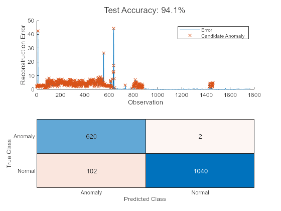
thresh = 0.55;
anomalies = errorAll > thresh*mean(errorAll);

helperVisualizeAnomalies(anomalies, errorAll, featureTest);
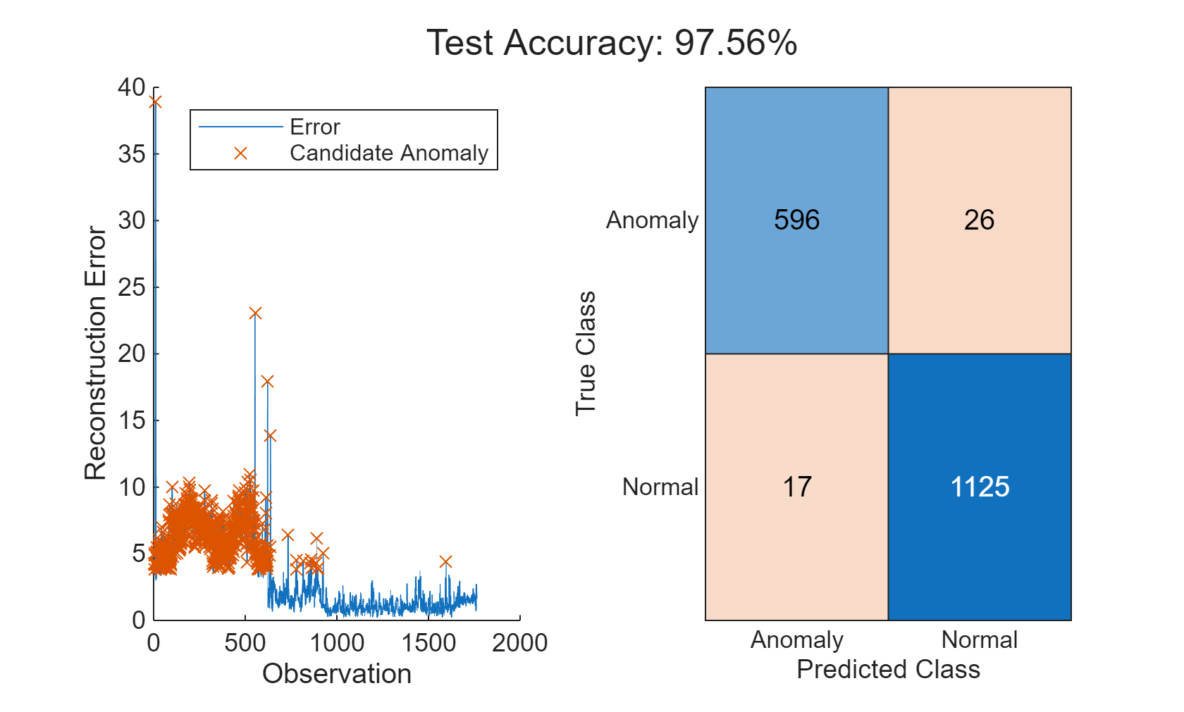
이 예제에서는 3개의 각기 다른 모델을 사용하여 이상을 감지합니다. 3개의 모델이 모두 높은 정확도와 낮은 오분류 비율로 이상을 감지할 수 있습니다. 여러 모델의 상대적인 성능은 다른 특징 세트를 선택하거나 각 모델에 다른 하이퍼파라미터를 사용하는 경우 바뀔 수 있습니다. 진단 특징 디자이너 MATLAB 앱을 사용하여 특징 선택을 추가로 시험해 보십시오.
지원 함수
function E = helperCalculateError(X, Y)
% HELPERCALCULATEERROR calculates the rms error value between the
% inputs X, Y
E = zeros(length(X),1);
for i = 1:length(X)
   E(i,:) = sqrt(sum((Y{i} - X{i}).^2));
end

end

function helperVisualizeError(errorBefore, errorAfter)
% HELPERVISUALIZEERROR creates a plot to visualize the errors on detecting
% before and after conditions
figure("Color", "W")
tiledlayout("flow")

nexttile
plot(1:length(errorBefore), errorBefore, 'LineWidth',1.5), grid on
title(["Before Maintenance", ...
   sprintf("Mean Error: %.2f\n", mean(errorBefore))])
xlabel("Observations")
ylabel("Reconstruction Error")
ylim([0 15])

nexttile
plot(1:length(errorAfter), errorAfter, 'LineWidth',1.5), grid on,
title(["After Maintenance", ...
   sprintf("Mean Error: %.2f\n", mean(errorAfter))])
xlabel("Observations")
ylabel("Reconstruction Error")
ylim([0 15])

end

function helperVisualizeAnomalies(anomalies, errorAll, featureTest)
% HELPERVISUALIZEANOMALIES creates a plot of the detected anomalies
anomalyIdx = find(anomalies);
anomalyErr = errorAll(anomalies);

predAE = categorical(anomalies, [1, 0], ["Anomaly", "Nominal"]);
trueAE = renamecats(featureTest.label,["Before","After"],["Anomaly","Nominal"]);

acc = numel(find(trueAE == predAE))/numel(predAE)*100;
figure;
t = tiledlayout("flow");
title(t, "Test Accuracy: " + round(mean(acc),2) + "%");
nexttile
hold on
plot(errorAll)
plot(anomalyIdx, anomalyErr, 'x')
hold off
ylabel("Reconstruction Error")
xlabel("Observation")
legend("Error", "Candidate Anomaly")

nexttile
confusionchart(trueAE,predAE)

end

function helperVisualizeModelBehavior(normalData, abnormalData, reconstructedNorm, reconstructedAbNorm)
%HELPERVISUALIZEMODELBEHAVIOR Visualize model behavior on sample validation data

figure("Color", "W")
tiledlayout("flow")

nexttile()
hold on
colororder('default')
yyaxis left
plot(normalData')
plot(reconstructedNorm',":","LineWidth",1.5)
hold off
title("Nominal Input")
grid on
ylabel("Feature Value")
yyaxis right
stem(abs(normalData' - reconstructedNorm'))
ylim([0 2])
ylabel("Error")
legend(["Input", "Reconstructed","Error"],"Location","southwest")

nexttile()
hold on
yyaxis left
plot(abnormalData)
plot(reconstructedAbNorm',":","LineWidth",1.5)
hold off
title("Abnormal Input")
grid on
ylabel("Feature Value")
yyaxis right
stem(abs(abnormalData' - reconstructedAbNorm'))
ylim([0 2])
ylabel("Error")
legend(["Input", "Reconstructed","Error"],"Location","southwest")

end

function X = helperExtractLabeledData(featureTable, label)
%HELPEREXTRACTLABELEDDATA Extract data from before or after operating
%conditions and re-format to support input to biLSTM network

% Select data with label After
if label == "All"
   Xtemp = featureTable(:, 2:end).Variables;
else
   tF = featureTable.label == label;
   Xtemp = featureTable(tF, 2:end).Variables;
end

% Arrange data into cells
X = cell(length(Xtemp),1);
for i = 1:length(Xtemp)
   X{i,:} = Xtemp(i,:)';
end

end
참고 항목
cvpartition | OneClassSVM | fitcsvm | iforest | 진단 특징 디자이너