tsaresidual

Residual signal of a time-synchronous averaged signal

Syntax

Y = tsaresidual(X,fs,rpm,orderList)

Y = tsaresidual(X,t,rpm,orderList)

Y = tsaresidual(XT,rpm,orderList)

[Y,S] = tsaresidual(___)

___ = tsaresidual(___,Name,Value)

tsaresidual(___)

Description

Y = tsaresidual(X,fs,rpm,orderList) computes the residual signal Y of the time-synchronous averaged (TSA) signal vector X using sampling rate fs, the rotational speed rpm, and the orders to be filtered orderList. The residual signal is computed by removing the components in orderList and their harmonics from X. You can use Y to further extract condition indicators of rotating machinery for predictive maintenance. For example, extracting the root-mean-squared value of the residual signal is useful in identifying changes over time which indicate potential machine faults.

Y = tsaresidual(X,t,rpm,orderList) computes the residual signal Y of the TSA signal vector X with corresponding time values in vector t.

Y = tsaresidual(XT,rpm,orderList) computes the residual signal Y of the TSA signal stored in the timetable XT. XT must contain a single numeric column variable.

[Y,S] = tsaresidual(___) returns the amplitude spectrum S of the residual signal Y. S is the amplitude spectrum computed using the normalized fast Fourier transform (FFT) of Y.

___ = tsaresidual(___,Name,Value) allows you to specify additional parameters using one or more name-value pair arguments. You can use this syntax with any of the previous input and output arguments.

tsaresidual(___) with no output arguments plots the time-domain and frequency-domain plots of the raw and residual TSA signals.

Examples

Find and Visualize the Residual Signal of a Compound TSA Signal

Consider a drivetrain with six gears driven by a motor that is fitted with a vibration sensor, as depicted in the figure below. Gear 1 on the motor shaft meshes with gear 2 with a gear ratio of 17:1. The final gear ratio, that is, the ratio between gears 1 and 2 and gears 3 and 4, is 51:1. Gear 5, also on the motor shaft, meshes with gear 6 with a gear ratio of 10:1. The motor is spinning at 180 RPM, and the sampling rate of the vibration sensor is 50 KHz. To obtain the signal containing just the meshing components for gears 5 and 6, filter out the signal components due to the gears 1 and 2 and, 3 and 4 by specifying their gear ratios of 17 and 51 in orderList. The signal components corresponding to the shaft rotation (order = 1) is always implicitly included in the computation.

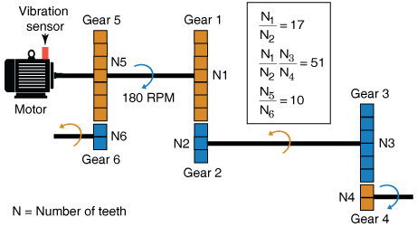
rpm = 180;                                          
fs = 50e3;                                          
t = (0:1/fs:(1/3)-1/fs)';                           % sample times
orderList = [17 51];                                
f = rpm/60*[1 orderList 10];

In practice, you would use measured data such as vibration signals obtained from an accelerometer. For this example, generate TSA signal X, which is the simulated data from the vibration sensor mounted on the motor.

X = sin(2*pi*f(1)*t) + sin(2*pi*2*f(1)*t) + ...     % motor shaft rotation and harmonic
    3*sin(2*pi*f(2)*t) + 3*sin(2*pi*2*f(2)*t) + ... % gear mesh vibration and harmonic for gears 1 and 2
    4*sin(2*pi*f(3)*t) + 4*sin(2*pi*2*f(3)*t) + ... % gear mesh vibration and harmonic for gears 3 and 4
    2*sin(2*pi*10*f(1)*t);                          % gear mesh vibration for gears 5 and 6

Compute the residual of the TSA signal using the sample time, rpm, and the mesh orders to be filtered out.

Y = tsaresidual(X,t,rpm,orderList);

The output Y is a vector containing the gear mesh signal and harmonics for gears 5 and 6.

Visualize the residual signal, the raw TSA signal, and their amplitude spectrum on a plot.

tsaresidual(X,fs,rpm,orderList)

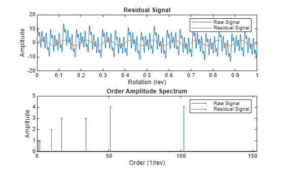
From the amplitude spectrum plot, observe the following components:

• The filtered component at the 17th order and its harmonic at the 34th order

• The second filtered component at the 51st order and its harmonic at the 102nd order

• The residual mesh components for gears 5 and 6 at the 10th order

• The filtered shaft component at the 1st and 2nd orders

• The amplitudes on the spectrum plot match the amplitudes of individual signals

Compute Residual Signal and Amplitude Spectrum of a TSA Signal

In this example, sineWavePhaseMod.mat contains the data of a phase modulated sine wave. XT is a timetable with the sine wave data and rpm used is 60 RPM. The sine wave has a frequency of 32 Hz, and to filter out the unmodulated sine wave, use 32 as the orderList.

Load the data and the required variables.

load('sineWavePhaseMod.mat','XT','rpm','orders')
head(XT,4)

         Time          Data  
    ______________    _______

    0 sec                   0
    0.00097656 sec     0.2011
    0.0019531 sec     0.39399
    0.0029297 sec     0.57078

Note that the time values in XT are strictly increasing, equidistant, and finite.

Compute the residual signal and its amplitude spectrum. Set the value of 'Domain' to 'frequency' since the orders are in Hz.

[Y,S] = tsaresidual(XT,rpm,orders,'Domain','frequency')

Y=1024×1 timetable
         Time           Data   
    ______________    _________

    0 sec             2.552e-15
    0.00097656 sec     0.051822
    0.0019531 sec       0.10116
    0.0029297 sec       0.14566
    0.0039062 sec       0.18317
    0.0048828 sec       0.21188
    0.0058594 sec       0.23039
    0.0068359 sec       0.23776
    0.0078125 sec        0.2336
    0.0087891 sec       0.21803
    0.0097656 sec       0.19174
    0.010742 sec         0.1559
    0.011719 sec        0.11215
    0.012695 sec       0.062503
    0.013672 sec      0.0092782
    0.014648 sec      -0.045032
      ⋮

S = 1024×1 complex

  -0.0000 + 0.0000i
   0.0000 + 0.0000i
   0.0000 + 0.0000i
   0.0000 + 0.0000i
   0.0000 + 0.0000i
  -0.0000 - 0.0000i
  -0.0000 + 0.0000i
   0.0000 + 0.0000i
  -0.0000 - 0.0000i
   0.0000 + 0.0000i
      ⋮

The output Y is a timetable that contains the residual signal, that is, the phase modulation signal, while S is a vector that contains the amplitude spectrum of the residual signal Y.

Visualize the Residual and Amplitude Spectrum of a TSA Signal

In this example, sineWaveAmpMod.mat contains the data of an amplitude modulated sine wave. X is a vector with the amplitude modulated sine wave data obtained at a shaft speed of 60 RPM. The unmodulated sine wave has a frequency of 32 Hz and amplitude of 1.0 units.

Load the data, and plot the residual signal of the amplitude modulated TSA signal X. To obtain the residual signal, filter out the unmodulated sine wave by specifying the frequency of 32 Hz in orderList. Set the value of 'Domain' to 'frequency'.

load('sineWaveAmpMod.mat','X','t','rpm','orderList')
tsaresidual(X,t,rpm,orderList,'Domain','frequency');

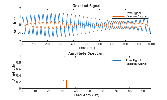
From the plot, observe the waveform and amplitude spectrum of the residual and raw signals, respectively.

Input Arguments

X — Time-synchronous averaged (TSA) signal

vector

Time-synchronous averaged (TSA) signal, specified as a vector. The time-synchronous averaged signal is computed from a long and relatively periodic raw signal through synchronization, resampling, and averaging. For more information on TSA signals, see tsa.

Time-synchronous averaging is a convenient method of background noise reduction in a spectrum of complex signals. It is effective in concentrating useful information that can be extracted from a time-domain signal for predictive maintenance. The synchronization typically requires a tachometer pulse signal in addition to the raw sensor data. The TSA signal depicts measurements at equally spaced angular positions over a single revolution of a shaft of interest.

XT — Time-synchronous averaged signal

timetable

Time synchronous averaged (TSA) signal, specified as a timetable. XT must contain a single numeric column variable corresponding to the TSA signal. Time values in XT must be strictly increasing, equidistant, and finite.

fs — Sampling frequency of the TSA signal

positive scalar

Sampling frequency of the TSA signal in Hertz, specified as a positive scalar.

t — Sample times of the TSA signal

positive scalar | vector of positive values

Sample times of the TSA signal, specified as a positive scalar or a vector of positive values.

If t is:

• A positive scalar, it contains the time interval or duration between samples. You must specify t as a duration variable.

• A vector of positive values, it contains sample times corresponding to elements in X. The time values must be strictly increasing, equidistant, and finite. You can specify t as a double or duration variable.

rpm — Rotational speed of the shaft

positive scalar

Rotational speed of the shaft, specified as a positive scalar. tsaresidual uses a bandwidth equal to the shaft speed around the frequencies of interest to filter out the undesired frequency components from the TSA signal. The signal components corresponding to this frequency, that is, order = 1 are always filtered out.

Specify rpm in revolutions per minute.

orderList — Orders to be filtered out of the TSA signal

vector of positive values

Orders to be filtered out of the TSA signal, specified as a vector of positive values. Select the orders and harmonics to be filtered out of the TSA signal by observing them on the amplitude spectrum plot. For instance, specify orderList as the known mesh orders in a gear train to filter out the known components and their harmonics. For more information, see Find and Visualize the Residual Signal of a Compound TSA Signal. Specify the units of orderList by selecting the appropriate value for 'Domain'.

Name-Value Arguments

Specify optional pairs of arguments as Name1=Value1,...,NameN=ValueN, where Name is the argument name and Value is the corresponding value. Name-value arguments must appear after other arguments, but the order of the pairs does not matter.

Before R2021a, use commas to separate each name and value, and enclose Name in quotes.

Example: …,'NumRotations',5

NumHarmonics — Number of shaft and gear meshing frequency harmonics to be filtered

2 (default) | positive integer

Number of shaft and gear meshing frequency harmonics to be filtered, specified as the comma-separated pair consisting of 'NumHarmonics' and a positive integer. Modify 'NumHarmonics' if your TSA signal contains more than two known harmonics of components to be filtered.

NumRotations — Number of shaft rotations in the TSA signal

1 (default) | positive integer

Number of shaft rotations in the TSA signal, specified as the comma-separated pair consisting of 'NumRotations' and a positive integer. Modify 'NumRotations' if your input X or XT contains data for more than one rotation of the driver gear shaft. The function uses 'NumRotations' to determine the number of rotations to be shown on the x-axis of the plot. The filtering results in Y are not affected by this value.

Domain — Units of the orderList values

'order' (default) | 'frequency'

Units of the orderList values, specified as the comma-separated pair consisting of 'Domain' and one of the following:

• 'frequency', if the orders in orderList are specified as frequencies in units of Hertz.

• 'order', if the orders in orderList are specified as number of rotations relative to the value of rpm. For example, if the rotational speed of the driven gear is defined as a factor of the driver gear rpm, specify 'Domain' as 'order'. Also, choose 'order' if you are comparing data obtained from machines operating at different speeds.

Output Arguments

Y — Residual signal of the TSA signal

vector | timetable

Residual signal of the TSA signal, returned as:

• A vector, when the TSA signal is specified as a vector X

• A timetable, when the TSA signal is specified as a timetable XT

The residual signal is computed by removing the components in orderList and the shaft signal along with their respective harmonics from X. You can use Y to further extract condition indicators of rotating machinery for predictive maintenance. For example, extracting the root-mean-squared value of the residual signal is useful in identifying changes over time, which indicate potential machine faults. For more information on how Y is computed, see Algorithms.

S — Amplitude spectrum of the residual signal

vector

Amplitude spectrum of the residual signal, returned as a vector. S is the normalized fast Fourier transform of the signal Y. S has the same length as the input TSA signal X. For more information on how S is computed, see Algorithms.

Algorithms

Residual Signal

The residual signal is computed from the TSA signal by removing the following from the signal spectrum:

• Shaft frequency and its harmonics

• Gear meshing frequencies and their harmonics

The frequencies are removed by computing the discrete Fourier transform (DFT) and setting the spectrum values to zero at the specified frequencies. tsaresidual uses a bandwidth equal to the shaft speed around the frequencies of interest to filter out the undesired frequency components, as mentioned in [4].

Amplitude Spectrum

The amplitude spectrum of the residual signal is computed as follows,

$$\text{S = }\frac{\text{fft}(Y)}{\text{length}(Y)*2}$$

Here, Y is the residual signal.

References

[1] McFadden, P.D. "Examination of a Technique for the Early Detection of Failure in Gears by Signal Processing of the Time Domain Average of the Meshing Vibration." Aero Propulsion Technical Memorandum 434. Melbourne, Australia: Aeronautical Research Laboratories, Apr. 1986.

[2] Večeř, P., Marcel Kreidl, and R. Šmíd. "Condition Indicators for Gearbox Monitoring Systems." Acta Polytechnica 45.6 (2005), pages 35-43.

[3] Zakrajsek, J. J., Townsend, D. P., and Decker, H. J. "An Analysis of Gear Fault Detection Methods as Applied to Pitting Fatigue Failure Data." Technical Memorandum 105950. NASA, Apr. 1993.

[4] Zakrajsek, James J. "An investigation of gear mesh failure prediction techniques." National Aeronautics and Space Administration Cleveland OH Lewis Research Center, 1989. No. NASA-E-5049.

Extended Capabilities

C/C++ Code Generation

Generate C and C++ code using MATLAB® Coder™.

Usage notes and limitations:

• Syntaxes that generate plots are not supported for code generation.

Version History

Introduced in R2018b