Main Content

predictRUL

Estimate remaining useful life for a test component

Description

The predictRUL function estimates the remaining useful life (RUL) of a test component given an estimation model and information about its usage time and degradation profile. Before predicting the RUL, you must first configure your estimation model using historical data regarding the health of an ensemble of similar components, such as multiple machines manufactured to the same specifications. To do so, use the fit function.

Using predictRUL, you can estimate the remaining useful life for the following types of estimation models:

  • Degradation models

  • Survival models

  • Similarity models

For a basic example illustrating RUL prediction, see Update RUL Prediction as Data Arrives.

For general information on predicting remaining useful life using these models, see RUL Estimation Using RUL Estimator Models.

estRUL = predictRUL(mdl,data) estimates the remaining useful life for a component using similarity model mdl and the degradation feature profiles in data. data contains feature measurements over the life span of the component up to the current life time.

example

estRUL = predictRUL(mdl,data,bounds) estimates the remaining useful life for a component using a similarity model and the feature bounds specified in bounds.

estRUL = predictRUL(mdl,threshold) estimates the RUL for a component using degradation model mdl and the current life time variable value stored in mdl. The RUL is the remaining time before the forecast response of the model reaches the threshold value threshold.

example

estRUL = predictRUL(mdl,usageTime) estimates the RUL for a component using reliability survival model mdl and the current usage time for the component.

example

estRUL = predictRUL(mdl,covariates) estimates the RUL of a component using covariate survival model mdl and the current covariate values for the component.

example

estRUL = predictRUL(___,Name,Value) specifies additional options using one or more name-value pair arguments.
example

[estRUL,ciRUL] = predictRUL(___) returns the confidence interval associated with the RUL estimation.

[estRUL,ciRUL,pdfRUL] = predictRUL(___) returns the probability density function for the RUL estimation.

example

[estRUL,ciRUL,pdfRUL,histRUL] = predictRUL(___) returns the histogram of component similarity scores when estimating RUL using a similarity model.

Examples

collapse all

Load training data.

load('pairwiseTrainTables.mat')

The training data is a cell array of tables. Each table is a degradation feature profile for a component. Each profile consists of life time measurements in the "Time" variable and corresponding degradation feature measurements in the "Condition" variable.

Create a pairwise similarity model that computes distance using dynamic time warping with an absolute distance metric and uses hours as a life time unit.

mdl = pairwiseSimilarityModel('Method',"dtw",'Distance',"absolute",'LifeTimeUnit',"hours");

Train the similarity model using the training data. Specify the names of the life time and data variables.

fit(mdl,pairwiseTrainTables,"Time","Condition")

Load testing data. The test data contains the degradation feature measurements for a test component up to the current life time.

load('pairwiseTestData.mat')

Predict the RUL of the test component using the trained similarity model.

estRUL = predictRUL(mdl,pairwiseTestData)
estRUL = duration
   93.671 hr

The estimated RUL for the component is around 94 hours.

Load observation data.

load('linTestData.mat','linTestData1')

For this example, assume that the training data is not historical data, but rather real-time observations of the component condition.

Based on knowledge of the degradation feature limits, define a threshold condition indicator value that indicates the end-of-life of a component.

threshold = 60;

Create a linear degradation model arbitrary prior distribution data and a specified noise variance. Also, specify the life time and data variable names for the observation data.

mdl = linearDegradationModel('Theta',1,'ThetaVariance',1e6,'NoiseVariance',0.003,...
                             'LifeTimeVariable',"Time",'DataVariables',"Condition",...
                             'LifeTimeUnit',"hours");

Observe the component condition for 50 hours, updating the degradation model after each observation.

for i=1:50
    update(mdl,linTestData1(i,:));
end

After 50 hours, predict the RUL of the component using the current life time value stored in the model.

estRUL = predictRUL(mdl,threshold)
estRUL = duration
   50.301 hr

The estimated RUL is about 50 hours, which indicates a total predicted life span of about 100 hours.

Load training data.

load('expTrainTables.mat')

The training data is a cell array of tables. Each table is a degradation feature profile for a component. Each profile consists of life time measurements in the "Hours" variable and corresponding degradation feature measurements in the "Condition" variable.

Create an exponential degradation model, specifying the life time variable units.

mdl = exponentialDegradationModel('LifeTimeUnit',"hours");

Train the degradation model using the training data. Specify the names of the life time and data variables.

fit(mdl,expTrainTables,"Time","Condition")

Load testing data, which is a run-to-failure degradation profile for a test component. The test data is a table with the same life time and data variables as the training data.

load('expTestData.mat')

Based on knowledge of the degradation feature limits, define a threshold condition indicator value that indicates the end-of-life of a component.

threshold = 500;

Assume that you measure the component condition indicator every hour for 150 hours. Update the trained degradation model with each measurement. Then, predict the remaining useful life of the component at 150 hours. The RUL is the forecasted time at which the degradation feature will pass the specified threshold.

for t = 1:150 
 update(mdl,expTestData(t,:)) 
end 
estRUL = predictRUL(mdl,threshold) 
estRUL = duration
   136.45 hr

The estimated RUL is around 137 hours, which indicates a total predicted life span of 287 hours.

Load training data.

load('covariateData.mat')

This data contains battery discharge times and related covariate information. The covariate variables are:

  • Temperature

  • Load

  • Manufacturer

The manufacturer information is a categorical variable that must be encoded.

Create a covariate survival model, and train it using the training data.

mdl = covariateSurvivalModel('LifeTimeVariable',"DischargeTime",'LifeTimeUnit',"hours",...
   'DataVariables',["Temperature","Load","Manufacturer"],'EncodedVariables',"Manufacturer");
fit(mdl,covariateData)
Successful convergence: Norm of gradient less than OPTIONS.TolFun

Suppose you have a battery pack manufactured by maker B that has run for 30 hours. Create a test data table that contains the usage time, DischargeTime, and the measured ambient temperature, TestAmbientTemperature, and current drawn, TestBatteryLoad.

TestBatteryLoad = 25;
TestAmbientTemperature = 60; 
DischargeTime = hours(30);
TestData = timetable(TestAmbientTemperature,TestBatteryLoad,"B",'RowTimes',hours(30));
TestData.Properties.VariableNames = {'Temperature','Load','Manufacturer'};
TestData.Properties.DimensionNames{1} = 'DischargeTime';

Predict the RUL for the battery.

estRUL = predictRUL(mdl,TestData)
estRUL = duration
   38.332 hr

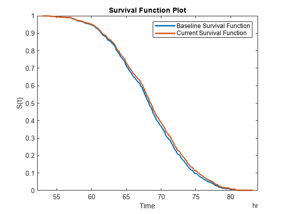
Plot the survival function for the covariate data of the battery.

plot(mdl,TestData)

Figure contains an axes object. The axes object with title Survival Function Plot, xlabel Time, ylabel S(t) contains 2 objects of type stair. These objects represent Baseline Survival Function, Current Survival Function.

Load training data.

load('reliabilityData.mat')

This data is a column vector of duration objects representing battery discharge times.

Create a reliability survival model, specifying the life time variable and life time units.

mdl = reliabilitySurvivalModel('LifeTimeVariable',"DischargeTime",'LifeTimeUnit',"hours");

Train the survival model using the training data.

fit(mdl,reliabilityData)

Predict the life span of a new component, and obtain the probability distribution function for the estimate.

[estRUL,ciRUL,pdfRUL] = predictRUL(mdl);

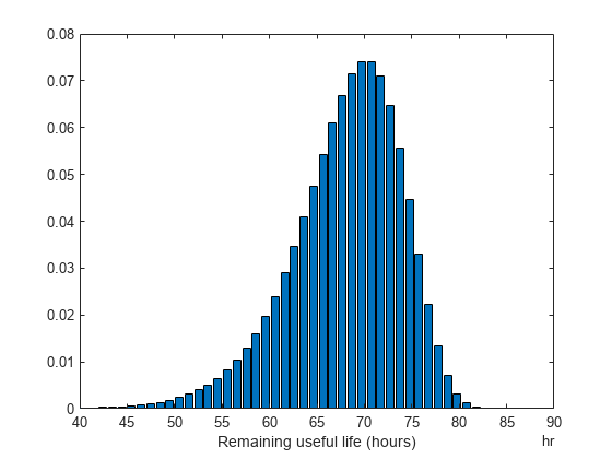
Plot the probability distribution.

bar(pdfRUL.RUL,pdfRUL.ProbabilityDensity)
xlabel('Remaining useful life (hours)')
xlim(hours([40 90]))

Figure contains an axes object. The axes object with xlabel Remaining useful life (hours) contains an object of type bar.

Improve the distribution view by providing the number of bins and bin size for the prediction.

[estRUL,ciRUL,pdfRUL] = predictRUL(mdl,'BinSize',0.5,'NumBins',500);
bar(pdfRUL.RUL,pdfRUL.ProbabilityDensity)
xlabel('Remaining useful life (hours)')
xlim(hours([40 90]))

Figure contains an axes object. The axes object with xlabel Remaining useful life (hours) contains an object of type bar.

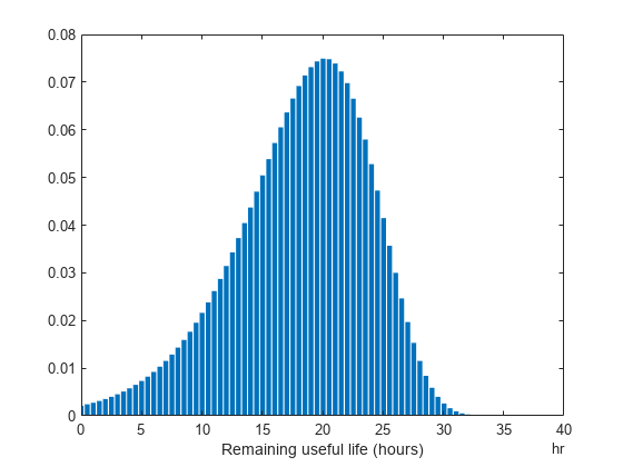
Predict the RUL for a component that has been operating for 50 hours.

[estRUL,ciRUL,pdfRUL] = predictRUL(mdl,hours(50),'BinSize',0.5,'NumBins',500);
bar(pdfRUL.RUL,pdfRUL.ProbabilityDensity)
xlabel('Remaining useful life (hours)')
xlim(hours([0 40]))

Figure contains an axes object. The axes object with xlabel Remaining useful life (hours) contains an object of type bar.

Input Arguments

collapse all

Remaining useful life prediction model, specified as one of the following models.

For more information on the different model types and when to use them, see Models for Predicting Remaining Useful Life.

Degradation feature profiles for estimating the RUL using similarity models, measured over the life span of a component up to its current life time, specified as one of the following:

  • N-by-(Mi+1) arrays, where N is the number of feature measurements (at different usage times) and Mi is the number of features. The first column contains the usage times and the remaining columns contain the corresponding measurements for degradation features. The order of the features must match the order specified in the DataVariables property of mdl.

  • table or timetable object. The table must contain variables with names that match the strings in the DataVariables and LifeTimeVariable properties of mdl.

data applies when mdl is a hashSimilarityModel, pairwiseSimilarityModel, or residualSimilarityModel, object.

Degradation feature bounds, which indicate the effective life span of a component, specified as an N-by-2 array, where N is the number of degradation features. For the ith feature, bounds(i,1) is the lower bound on the feature and bounds(i,2) is the upper bound. The order of the features must match the order specified in the DataVariables property of mdl.

Select bounds based on your knowledge of the allowable bounds for the degradation features.

bounds applies when mdl is a hashSimilarityModel, pairwiseSimilarityModel, or residualSimilarityModel object.

Data variable threshold limits for degradation models, specified as a scalar value. The remaining useful life is the remaining time before the forecasted response of the model reaches the threshold value.

The sign of the Theta property of mdl indicates the direction of degradation growth. If Theta is:

  • Positive, then threshold is an upper bound on the degradation feature

  • Negative, then threshold is a lower bound on the degradation feature

Select threshold based on your knowledge of the allowable bounds for the degradation feature.

threshold applies when mdl is a linearDegradationModel or exponentialDesgradationModel object.

Current usage time of the component, specified as a scalar value or a duration object. The units of usageTime must be compatible with the LifeTimeUnit property of mdl.

Current covariate values and usage time for the component, specified as a:

  • Row vector whose first column contains the usage time. The remaining columns specify the component covariate values only and not the life time values. The number of covariate values must match the number and order of the covariate data columns used when estimating mdl using fit.

  • table or timetable with one row. The table must contain the variables specified in the LifeTimeVariable, DataVariables, and CensorVariable properties of mdl.

If the covariate data contains encoded variables, then you must specify covariates using a table or timetable.

Name-Value Arguments

Specify optional pairs of arguments as Name1=Value1,...,NameN=ValueN, where Name is the argument name and Value is the corresponding value. Name-value arguments must appear after other arguments, but the order of the pairs does not matter.

Before R2021a, use commas to separate each name and value, and enclose Name in quotes.

Example: Alpha,0.2 sets the prediction confidence interval to the 0.2/2 to 1-0.2/2 percentile region.

Confidence level for computing ciRUL, specified as the comma-separated pair consisting of 'Alpha' and a scalar value in the range 0–1. predictRUL computes the confidence interval as the Alpha/2 to 1-Alpha/2 percentile region.

Number of bins used to evaluate pdfRUL, specified as the comma-separated pair consisting of 'NumBins' and a positive integer. This argument applies when mdl is a degradation model or survival model.

Bin size used to determine the life span for computing pdfRUL, specified as the comma-separated pair consisting of 'BinSize' and either a positive scalar or a duration object. This argument applies when mdl is a degradation model or reliability survival model.

Survival function conversion method for generating the probability density function of a covariate survival model, specified as the comma-separated pair consisting of 'Method' and one of the following:

  • 'empirical' — Generate pdfRUL by finding the gradient of the empirical cumulative distribution function. The cumulative distribution function is 1-S(t), where S(t) is the survival function.

  • 'weibull' — Generate pdfRUL by fitting a Weibull distribution to the survival function.

For more information on survival functions, see covariateSurvivalModel.

Output Arguments

collapse all

Estimated remaining useful life of a component, returned as a scalar. The returned value is in the units of the life time variable as indicated by the LifeTimeUnit property of mdl.

Confidence interval associated with estRUL, returned as a two-element row vector. Specify the percentile for the confidence interval using Alpha.

RUL probability density function, returned as a timetable if the life time variable of mdl is time-based, or as a table otherwise.

The life span used by predictRUL when computing the probability density function depends on the type of RUL model you specify. If mdl is a:

  • Degradation model, then the life span is [usageTime usageTime+BinSize*NumBins].

  • Reliability survival model, then the life span is [T T+BinSize*NumBins], where T is the usage time specified in usageTime.

  • Covariate survival model, then the life span is linspace(T1,T2,NumBins), where [T1,T2] is the life range of components as determined by the BaslineCumulativeHazard property of mdl.

  • Similarity model, then the life span depends on the life spans of the nearest neighbors found by the search algorithm. For example, if the NumNearestNeighbors property of mdl is 10 and the 10 nearest neighbors have life times in the range of 10 months to three years, then the histogram of failure times is found across this range. predictRUL then fits a probability density function to the raw histogram data using a kernel smoothing approach.

Raw similarity scores for histogram plotting, returned as a timetable if the life time variable of mdl is time-based, or as a table otherwise. histRUL has the following variables:

  • 'RUL' — Remaining useful life values of historical components used to fit the parameters of mdl.

  • 'NormalizedDistanceScore' — Similarity scores obtained by comparing the test component to the historical components used to fit the parameters of mdl.

The histogram of the data in histRUL is the unfitted version of pdfRUL. To plot the histogram, at the MATLAB® command line, type:

bar(histRUL.RUL,histRUL.NormalizedDistanceScore)

histRUL is returned when mdl is a hashSimilarityModel, pairwiseSimilarityModel, or residualSimilarityModel object.

Extended Capabilities

Version History

Introduced in R2018a

expand all

Go to top of page