Obtain Best Feasible Point
R2026bThis example shows how to obtain the best feasible point encountered by fmincon.
The helper function bigtoleft is a cubic polynomial objective function in a three-dimensional variable x that grows rapidly negative as the x(1) coordinate becomes negative. Its gradient is a three-element vector. The code for the bigtoleft helper function appears at the end of this example.
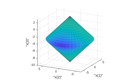
The constraint set for this example is the intersection of the interiors of two cones—one pointing up, and one pointing down. The constraint function is a two-component vector containing one component for each cone. Because this example is three-dimensional, the gradient of the constraint is a 3-by-2 matrix. The code for the twocone helper function appears at the end of this example.
Create a figure of the constraints colored using the objective function by calling the plottwoconecons function, whose code appears at the end of this example.
figure1 = plottwoconecons;
Create Options To Use Derivatives
To enable fmincon to use the objective gradient and constraint gradients, set appropriate options. Choose the "sqp" algorithm.
options = optimoptions("fmincon",Algorithm="sqp",...
    SpecifyConstraintGradient=true,SpecifyObjectiveGradient=true);
To examine the solution process, set options to return iterative display.
options.Display = "iter";Minimize Using Derivative Information
Set the initial point x0 = [-1/20,-1/20,-1/20].
x0 = -1/20*ones(1,3);
The problem has no linear constraints or bounds. Set those arguments to [].
A = [];
b = [];
Aeq = [];
beq = [];
lb = [];
ub = [];
Solve the problem.
[x,fval,eflag,output] = fmincon(@bigtoleft,x0,...
           A,b,Aeq,beq,lb,ub,@twocone,options);
Iter Func-count Fval Feasibility Step Length Norm of First-order Wall-Clock Time
step optimality
0 1 -1.625000e-03 0.000e+00 1.000e+00 0.000e+00 8.250e-02 0.030856 sec
1 3 -2.490263e-02 0.000e+00 1.000e+00 8.325e-02 5.449e-01 0.041235 sec
2 5 -2.529919e+02 0.000e+00 1.000e+00 2.802e+00 2.585e+02 0.043094 sec
3 7 -6.408576e+03 9.472e+00 1.000e+00 1.538e+01 1.771e+03 0.045334 sec
4 9 -1.743599e+06 5.301e+01 1.000e+00 5.991e+01 9.216e+04 0.047695 sec
5 11 -5.552305e+09 1.893e+03 1.000e+00 1.900e+03 1.761e+07 0.049181 sec
6 13 -1.462524e+15 5.632e+04 1.000e+00 5.636e+04 8.284e+10 0.050194 sec
7 15 -2.573346e+24 1.471e+08 1.000e+00 1.471e+08 1.058e+17 0.051450 sec
8 17 -1.467510e+41 2.617e+13 1.000e+00 2.617e+13 1.789e+28 0.052497 sec
9 19 -8.716877e+72 2.210e+24 1.000e+00 2.210e+24 2.387e+49 0.053538 sec
10 21 -5.598248e+134 4.090e+44 1.000e+00 4.090e+44 4.368e+90 0.054506 sec
11 23 -5.691634e+258 1.355e+86 1.000e+00 1.136e+86 1.967e+173 0.055508 sec
Objective function returned Inf; trying a new point...
12 300 -5.691634e+258 1.355e+86 1.766e-43 1.394e+141 1.967e+173 0.059191 sec
Feasible point with lower objective function value found, but optimality criteria not satisfied. See output.bestfeasible..
Solver stopped prematurely.
fmincon stopped because it exceeded the function evaluation limit,
options.MaxFunctionEvaluations = 3.000000e+02.
Examine Solution and Solution Process
Examine the solution, objective function value, exit flag, and number of function evaluations and iterations.
disp(x)
   1.0e+85 *

   -7.8891    7.7904   -2.4638
disp(fval)
-5.6916e+258
disp(eflag)
0
disp(output.constrviolation)
1.3551e+86
The objective function value is smaller than –1e250, a very negative value. The constraint violation is larger than 1e85, a large amount that is still much smaller in magnitude than the objective function value. The exit flag also shows that the returned solution is infeasible.
To recover the best feasible point that fmincon encounters, along with its objective function value, display the output.bestfeasible structure.
disp(output.bestfeasible)
                  x: [-2.9297 -0.1813 -0.1652]
               fval: -252.9919
    constrviolation: 0
      firstorderopt: 258.5032
The bestfeasible point is not a good solution, as you see in the next section. It is simply the best feasible point that fmincon encountered in its iterations. In this case, even though bestfeasible is not a solution, it is a better point than the returned infeasible solution.
table([fval;output.bestfeasible.fval],...
    [output.constrviolation;output.bestfeasible.constrviolation],...
    VariableNames=["Fval" "Constraint Violation"],...
    RowNames=["Final Point" "Best Feasible"])
ans = 2×2 table
                         Fval        Constraint Violation
                     ____________    ____________________

    Final Point      -5.6916e+258         1.3551e+86
    Best Feasible         -252.99                  0
The output.bestfeasible structure contains the best feasible point that fmincon encountered at the end of each of its iterations. In rare cases, it is possible that fmincon encounters a feasible point in some intermediate calculation that has an even lower objective function value than it reports.
Improve Solution: Set Bounds
There are several ways to obtain a feasible solution. One way is to set bounds on the variables.
lb = -10*ones(3,1);
ub = -lb;
[xb,fvalb,eflagb,outputb] = fmincon(@bigtoleft,x0,...
           A,b,Aeq,beq,lb,ub,@twocone,options);
Iter Func-count Fval Feasibility Step Length Norm of First-order Wall-Clock Time
step optimality
0 1 -1.625000e-03 0.000e+00 1.000e+00 0.000e+00 8.250e-02 0.017752 sec
1 3 -2.490263e-02 0.000e+00 1.000e+00 8.325e-02 5.449e-01 0.029418 sec
2 5 -2.529919e+02 0.000e+00 1.000e+00 2.802e+00 2.585e+02 0.030367 sec
3 7 -4.867942e+03 5.782e+00 1.000e+00 1.151e+01 1.525e+03 0.031345 sec
4 9 -1.035980e+04 3.536e+00 1.000e+00 9.587e+00 1.387e+03 0.032274 sec
5 12 -5.270030e+03 2.143e+00 7.000e-01 4.865e+00 2.804e+02 0.033399 sec
6 14 -2.538935e+03 2.855e-02 1.000e+00 2.229e+00 1.715e+03 0.034344 sec
7 16 -2.703318e+03 2.331e-02 1.000e+00 5.517e-01 2.521e+02 0.035426 sec
8 19 -2.845097e+03 0.000e+00 1.000e+00 1.752e+00 8.874e+01 0.036373 sec
9 21 -2.896933e+03 2.149e-03 1.000e+00 1.709e-01 1.608e+01 0.037296 sec
10 23 -2.894135e+03 7.953e-06 1.000e+00 1.039e-02 2.028e+00 0.038225 sec
11 25 -2.894126e+03 4.114e-07 1.000e+00 2.313e-03 2.100e-01 0.039188 sec
12 27 -2.894125e+03 4.618e-09 1.000e+00 2.450e-04 1.470e-04 0.040097 sec
Feasible point with lower objective function value found, but optimality criteria not satisfied. See output.bestfeasible..
Local minimum found that satisfies the constraints.
Optimization completed because the objective function is non-decreasing in
feasible directions, to within the value of the optimality tolerance,
and constraints are satisfied to within the value of the constraint tolerance.
<stopping criteria details>
The iterative display shows that fmincon starts at a feasible point (feasibility 0), spends a few iterations infeasible, again reaches 0 feasibility, then has small but nonzero infeasibility for the remaining iterations. The solver again reports that it found a lower feasible value at a point other than the final point xb. View the final point and objective function value, and the reported feasible point with lower objective function value.
disp(xb)
-6.5000 -0.0000 -3.5000
disp(fvalb)
-2.8941e+03
disp(outputb.bestfeasible)
                  x: [-6.5000 2.4498e-04 -3.5000]
               fval: -2.8941e+03
    constrviolation: 4.1139e-07
      firstorderopt: 0.2100
The constraint violation at the bestfeasible point is about 4.113e-7. In the iterative display, this infeasibility occurs at iteration 11. The reported objective function value at that iteration is -2.894126e3, which is slightly less than the final value of -2.894125e3. The final point has lower infeasibility and first-order optimality measure. Which point is better? They are nearly the same, but each point has some claim to being better. To see the solution details, set the display format to long.
format long
table([fvalb;outputb.bestfeasible.fval],...
    [outputb.constrviolation;outputb.bestfeasible.constrviolation],...
    [outputb.firstorderopt;outputb.bestfeasible.firstorderopt],...
    VariableNames=["Function Value" "Constraint Violation" "First-Order Optimality"],...
    RowNames=["Final Point" "Best Feasible"])
ans = 2×3 table
                      Function Value      Constraint Violation    First-Order Optimality
                     _________________    ____________________    ______________________

    Final Point      -2894.12500606353    4.61807037055451e-09     0.000146960596453027
    Best Feasible    -2894.12553469474    4.11390739252226e-07         0.21002648400065
Improve Solution: Use Another Algorithm
Another way to obtain a feasible solution is to use the "interior-point" algorithm, even without bounds,
lb = [];
ub = [];
options.Algorithm = "interior-point";
[xip,fvalip,eflagip,outputip] = fmincon(@bigtoleft,x0,...
           A,b,Aeq,beq,lb,ub,@twocone,options);
                                            First-order      Norm of
 Iter F-count            f(x)  Feasibility   optimality         step   Wall-Clock Time
    0       1   -1.625000e-03    0.000e+00    7.807e-02                   0.052219 sec
    1       2   -2.374253e-02    0.000e+00    5.222e-01    8.101e-02      0.101532 sec
    2       3   -2.232989e+02    0.000e+00    2.379e+02    2.684e+00      0.124709 sec
    3       4   -3.838433e+02    1.768e-01    3.198e+02    5.573e-01      0.128601 sec
    4       5   -3.115565e+03    1.810e-01    1.028e+03    4.660e+00      0.131850 sec
    5       6   -3.143463e+03    2.013e-01    8.965e+01    5.734e-01      0.142345 sec
    6       7   -2.917730e+03    1.795e-02    6.140e+01    5.231e-01      0.144765 sec
    7       8   -2.894095e+03    0.000e+00    9.206e+00    1.821e-02      0.146668 sec
    8       9   -2.894107e+03    0.000e+00    2.500e+00    3.899e-03      0.148019 sec
    9      10   -2.894142e+03    1.299e-05    2.136e-03    1.371e-02      0.150023 sec
   10      11   -2.894125e+03    3.614e-08    4.070e-03    1.739e-05      0.152057 sec
   11      12   -2.894125e+03    0.000e+00    5.994e-06    5.832e-08      0.165315 sec

Feasible point with lower objective function value found, but optimality criteria not satisfied. See output.bestfeasible..


Local minimum found that satisfies the constraints.

Optimization completed because the objective function is non-decreasing in
feasible directions, to within the value of the optimality tolerance,
and constraints are satisfied to within the value of the constraint tolerance.

<stopping criteria details>
The iterative display again shows fmincon reaching points that are infeasible in its search for a solution, and fmincon again issues a message that it encountered a feasible point with lower objective function value.
disp(xip)
-6.499999996950366 -0.000000032933162 -3.500000000098132
disp(fvalip)
-2.894124995999976e+03
disp(outputip.bestfeasible)
                  x: [-6.500000035892771 -7.634107877056255e-08 -3.500000000245461]
               fval: -2.894125047137579e+03
    constrviolation: 3.613823285064655e-08
      firstorderopt: 0.004069724066085
Again, the two solutions are nearly the same, and the bestfeasible solution comes from the iteration before the end. The final solution xip has better first-order optimality measure and feasibility, but the bestfeasible solution has slightly lower objective function value and an infeasibility that it not too large.
table([fvalip;outputip.bestfeasible.fval],...
    [outputip.constrviolation;outputip.bestfeasible.constrviolation],...
    [outputip.firstorderopt;outputip.bestfeasible.firstorderopt],...
    VariableNames=["Function Value" "Constraint Violation" "First-Order Optimality"],...
    RowNames=["Final Point" "Best Feasible"])
ans = 2×3 table
                      Function Value      Constraint Violation    First-Order Optimality
                     _________________    ____________________    ______________________

    Final Point      -2894.12499599998                       0     5.99383553128062e-06
    Best Feasible    -2894.12504713758    3.61382328506465e-08      0.00406972406608475
Finally, reset the format to the default short.
format shortHelper Functions
This code creates the bigtoleft helper function.
function [f,gradf] = bigtoleft(x)
% This is a simple function that grows rapidly negative
% as x(1) becomes negative.
%
f = 10*x(:,1).^3 + x(:,1).*x(:,2).^2 + x(:,3).*(x(:,1).^2 + x(:,2).^2);

if nargout > 1

   gradf=[30*x(1)^2+x(2)^2+2*x(3)*x(1);
       2*x(1)*x(2)+2*x(3)*x(2);
       (x(1)^2+x(2)^2)];

end
end
This code creates the twocone helper function.
function [ineqnonlin,eqnonlin,gradineqnonlin,gradeqnonlin] = twocone(x)
% This constraint is two cones, z > -10 + r
% and z < 3 - r.

eqnonlin = [];
r = sqrt(x(1)^2 + x(2)^2);
ineqnonlin = [-10+r-x(3);
    x(3)-3+r];

if nargout > 2

    gradeqnonlin = [];
    gradineqnonlin = [x(1)/r,x(1)/r;
       x(2)/r,x(2)/r;
       -1,1];

end
end
This code creates the function that plots the nonlinear constraints.
function figure1 = plottwoconecons
% Create figure
figure1 = figure;

% Create axes
axes1 = axes(Parent=figure1);
view([-63.5 18]);
grid("on");
hold("on");

% Set up polar coordinates and two cones
r = linspace(0,6.5,14);
th = 2*pi*linspace(0,1,40);
x = r'*cos(th);
y = r'*sin(th);
z = -10+sqrt(x.^2+y.^2);
zz = 3-sqrt(x.^2+y.^2);

% Evaluate objective function on cone surfaces
newxf = reshape(bigtoleft([x(:),y(:),z(:)]),14,40)/3000;
newxg = reshape(bigtoleft([x(:),y(:),z(:)]),14,40)/3000;

% Create lower surf with color set by objective
surf(x,y,z,newxf,Parent=axes1,EdgeAlpha=0.25);

% Create upper surf with color set by objective
surf(x,y,zz,newxg,Parent=axes1,EdgeAlpha=0.25);
axis equal
xlabel "x(1)"
ylabel "x(2)"
zlabel "x(3)"
end

