Explicit MPC Control of a Single-Input-Single-Output Plant
This example shows how to control a double integrator plant under input saturation in Simulink® using explicit MPC.
For an example that controls a double integrator with a traditional (implicit) MPC controller, see Model Predictive Control of a Single-Input-Single-Output Plant.
Define Plant Model
The linear open-loop dynamic model is a double integrator.
plant = tf(1,[1 0 0]);
Design MPC Controller
Create the controller object with a sample period of 0.1 seconds, and prediction and control horizons of 10 and 3 steps respectively.
Ts = 0.1;
mpcobj = mpc(plant, Ts, 10, 3);
-->"Weights.ManipulatedVariables" is empty. Assuming default 0.00000.
-->"Weights.ManipulatedVariablesRate" is empty. Assuming default 0.10000.
-->"Weights.OutputVariables" is empty. Assuming default 1.00000.
Specify actuator saturation limits as manipulated variable constraints.
mpcobj.MV = struct('Min',-1,'Max',1);
Explicit MPC
The constraints divide the state space of the MPC controller into many polyhedral regions such that within each region the MPC control law is a specific affine-in-the-state-and-reference function, with coefficients depending on the region. Explicit MPC calculates all these regions, and their relative control laws, offline. Online, the controller just selects and applies the precomputed solution relative to the current region, so it does not have to solve a constrained quadratic optimization problem at each control step. For more information on explicit MPC, see Explicit MPC.
Generate Explicit MPC Controller
Explicit MPC executes the equivalent explicit piecewise affine version of the MPC control law defined by the implicit MPC controller. To generate an explicit MPC controller from an implicit MPC controller, you must specify the range for each controller state, reference signal, manipulated variable and measured disturbance. Doing so ensures that the quadratic programming problem is solved in the space defined by these ranges. If at run time one of these independent variables falls outside of its range, the controller returns an error status and sets the manipulated variables to their last values. Therefore, it is important that you do not underestimate these ranges.
To generate suitable ranges, obtain some information on the controller states first. To display the controller initial states, use mpcstate.
mpcstate(mpcobj)
-->Converting the "Model.Plant" property to state-space.
-->Converting model to discrete time.
   Assuming no disturbance added to measured output #1.
-->"Model.Noise" is empty. Assuming white noise on each measured output.
MPCSTATE object with fields
          Plant: [0 0]
    Disturbance: [1×0 double]
          Noise: [1×0 double]
       LastMove: 0
     Covariance: [2×2 double]
As expected, the plant model used by the Kalman estimator has 2 states, and then there is one additional state needed to hold the last value of the manipulated variable.
MPC controller states include states from plant model, disturbance model noise model, and last values of the manipulated variables, in that order. To create a range structure where you can specify the range for each state, reference, and manipulated variable, use generateExplicitRange.
range = generateExplicitRange(mpcobj);
Setting the range of a state variable is sometimes difficult when the state does not correspond to a physical parameter. In that case, multiple runs of open-loop plant simulation with typical reference and disturbance signals, as well as model mismatches are recommended in order to collect data that reflect the ranges of states. For this example, overestimate the ranges as follows.
range.State.Min(:) = [-10;-10];
range.State.Max(:) = [10;10];
Usually you know the practical range of the reference signals being used at the nominal operating point in the plant. The ranges used to generate an explicit MPC controller must be at least as large as the practical range.
range.Reference.Min = -2;
range.Reference.Max = 2;
Specify the manipulated variable ranges. If the manipulated variables are constrained, the ranges used to generate the explicit MPC controller must be at least as large as these limits.
range.ManipulatedVariable.Min = -1.1;
range.ManipulatedVariable.Max = 1.1;
Use generateExplicitMPC command to obtain an explicit MPC controller with the specified parameter ranges.
mpcobjExplicit = generateExplicitMPC(mpcobj, range)
Regions found / unexplored:       19/       0


Explicit MPC Controller
---------------------------------------------
Controller sample time:    0.1 (seconds)
Polyhedral regions:        19
Number of parameters:      4
Is solution simplified:    No
State Estimation:          Default Kalman gain
---------------------------------------------
Type 'mpcobjExplicit.MPC' for the original implicit MPC design.
Type 'mpcobjExplicit.Range' for the valid range of parameters.
Type 'mpcobjExplicit.OptimizationOptions' for the options used in multi-parametric QP computation.
Type 'mpcobjExplicit.PiecewiseAffineSolution' for regions and gain in each solution.
Use the simplify function with the 'exact' method to join pairs of regions whose corresponding gains are the same and whose union is a convex set. Doing so can reduce memory footprint of the explicit MPC controller without sacrificing any performance.
mpcobjExplicitSimplified = simplify(mpcobjExplicit, 'exact')
Regions to analyze:       15/      15


Explicit MPC Controller
---------------------------------------------
Controller sample time:    0.1 (seconds)
Polyhedral regions:        15
Number of parameters:      4
Is solution simplified:    Yes
State Estimation:          Default Kalman gain
---------------------------------------------
Type 'mpcobjExplicitSimplified.MPC' for the original implicit MPC design.
Type 'mpcobjExplicitSimplified.Range' for the valid range of parameters.
Type 'mpcobjExplicitSimplified.OptimizationOptions' for the options used in multi-parametric QP computation.
Type 'mpcobjExplicitSimplified.PiecewiseAffineSolution' for regions and gain in each solution.
The number of piecewise affine regions has been reduced.
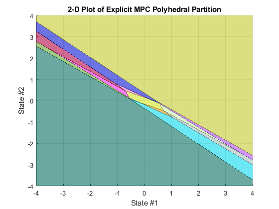
Plot Piecewise Affine Partition Along a Given Section
You can plot a 2-D section of the controller state space, and look at the regions in this section. For this example, plot the 2-D section of the state space defined by the first and second state variables (load angle and angular velocity). To do so you must first create a plot structure in which you fix all the other states (and reference signals) to specific values within their respective ranges.
To create a parameter structure where you can specify which 2-D section to plot afterward, use the generatePlotParameters function.
plotpars = generatePlotParameters(mpcobjExplicitSimplified)
plotpars =

  struct with fields:

                  State: [1×1 struct]
              Reference: [1×1 struct]
    MeasuredDisturbance: [1×1 struct]
    ManipulatedVariable: [1×1 struct]
In this example, you plot the first state variable against the second state variable. All the other parameters must be fixed at values within their respective ranges.
Leave the state variables free to vary, by not specifying indexes.
plotpars.State.Index = [];
plotpars.State.Value = [];
Specify index of the reference signal and fix it to a value of 0.
plotpars.Reference.Index = 1;
plotpars.Reference.Value = 0;
Specify index of the manipulated variable and fix it to a value of 0.
plotpars.ManipulatedVariable.Index = 1;
plotpars.ManipulatedVariable.Value = 0;
Use plotSection command to plot the 2-D section defined by the two free parameters. For more information, see plotSection.
plotSection(mpcobjExplicitSimplified, plotpars);
axis([-4 4 -4 4]);
grid
xlabel('State #1');
ylabel('State #2');
Simulate Using mpcmove Function
Compare closed-loop simulations for implicit and explicit MPC using the mpcmove and mpcmoveExplicit functions respectively.
Initialize variables to store the closed-loop MPC responses.
N = round(5/Ts);
YY = zeros(N,1);
YYExplicit = zeros(N,1);
UU = zeros(N,1);
UUExplicit = zeros(N,1);
Prepare the plant model used in simulation
sys = c2d(ss(plant),Ts);
xsys = [0;0];
xsysExplicit = xsys;
To obtain a pointer to the internal states for both controllers, use mpcstate.
xmpc = mpcstate(mpcobj);
xmpcExplicit = mpcstate(mpcobjExplicitSimplified);
Iteratively simulate the closed-loop response for both controllers.
for k = 1:N-1

    % update plant measurement
    ysys = sys.C*xsys;
    ysysExplicit = sys.C*xsysExplicit;

    % compute implicit MPC action
    u = mpcmove(mpcobj,xmpc,ysys,1);
    % compute explicit MPC action
    uExplicit = mpcmoveExplicit( ...
        mpcobjExplicit,xmpcExplicit,ysysExplicit,1);

    % store signals
    YY(k)=ysys;
    YYExplicit(k)=ysysExplicit;
    UU(k)=u;
    UUExplicit(k)=uExplicit;

    % update plant state
    xsys = sys.A*xsys + sys.B*u;
    xsysExplicit = sys.A*xsysExplicit + sys.B*uExplicit;
end

% Display norm of the differences between implicit and explicit controller signals.
fprintf(['\nDifference between implicit and' ...
    ' Explicit MPC responses using MPCMOVE command is %g\n'], ...
    norm(UU-UUExplicit)+norm(YY-YYExplicit));
Difference between implicit and Explicit MPC responses using MPCMOVE command is 1.30098e-13
Simulate Using sim Function
Compare closed-loop simulations between implicit and explicit MPC using the sim command.
N = 5/Ts;                      % number of simulation iterations
[y1,t1,u1] = sim(mpcobj,N,1);  % simulate with implicit MPC
[y2,t2,u2] = sim(mpcobjExplicitSimplified,N,1); % simulate with explicit MPC
-->Converting the "Model.Plant" property to state-space.
-->Converting model to discrete time.
   Assuming no disturbance added to measured output #1.
-->"Model.Noise" is empty. Assuming white noise on each measured output.
The simulation results are identical.
fprintf(['\nDifference between implicit and' ...
    ' Explicit MPC responses using SIM command is %g\n'], ...
    norm(u2-u1)+norm(y2-y1));
Difference between implicit and Explicit MPC responses using SIM command is 1.30316e-13
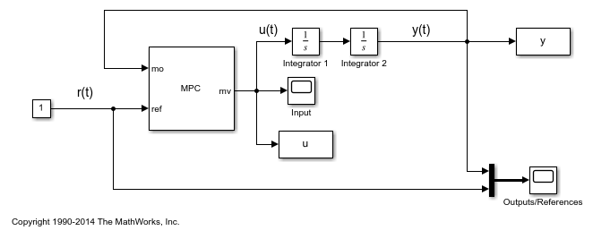
Simulate Using Simulink
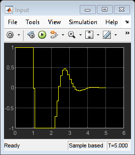
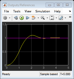
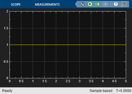
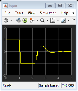
Simulate the implicit MPC controller in Simulink. The MPC Controller block is configured to use mpcobj as its controller. The scopes display the plant inputs and outputs.
mdl = 'mpc_doubleint';
open_system(mdl)
sim(mdl)
Simulate the explicit MPC controller in Simulink. The Explicit MPC Controller block is configured to use mpcobjExplicitSimplified as its controller. The scopes display the plant inputs and outputs, the current region, and the status.
mdlExplicit = 'empc_doubleint';
open_system(mdlExplicit)
sim(mdlExplicit)
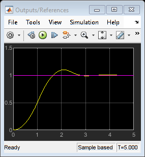
The closed-loop responses are identical.
fprintf(['\nDifference between implicit and' ...
    ' Explicit MPC responses in Simulink is %g\n'], ...
    norm(uExplicit-u)+norm(yExplicit-y));
Difference between implicit and Explicit MPC responses in Simulink is 1.3248e-13
See Also
Functions
generateExplicitMPC|generateExplicitRange|generateExplicitOptions|simplify|generatePlotParameters|plotSection|mpcmoveExplicit|sim
Objects
mpc|explicitMPC|mpcstate