geoimage
Description
The geoimage function displays RGB or grayscale images with
coordinates in any supported geographic or projected coordinate reference system (CRS). You
can display an image in a geographic axes or a map axes, which affects the map projection
that the function uses to display the data:
Geographic axes — A Web Mercator projection
Map axes — The projection specified by the
ProjectedCRSproperty of the map axes
geoimage(___, specifies
properties of the image using one or more name-value arguments in addition to any
combination of input arguments from the previous syntaxes. For a full list of
properties, see Image Properties.Name=Value)
im = geoimage(___)Image object. Use im to set properties after
creating the image. For a full list of properties, see Image Properties.
Examples
An RGB image is an m-by-n-by-3 array of RGB triplets. Each triplet defines a color for one element of the image.
Read a GeoTIFF image of Boston [1] into the workspace as an m-by-n-by-3 array of RGB triplets and a raster reference object.
[A,R] = readgeoraster("boston.tif");Display the image on a map. When the current axes is not a geographic or map axes, or when there is no current axes, the function displays the image in a new geographic axes.
figure
geoimage(A,R)
Add a title.
title("Boston Imagery")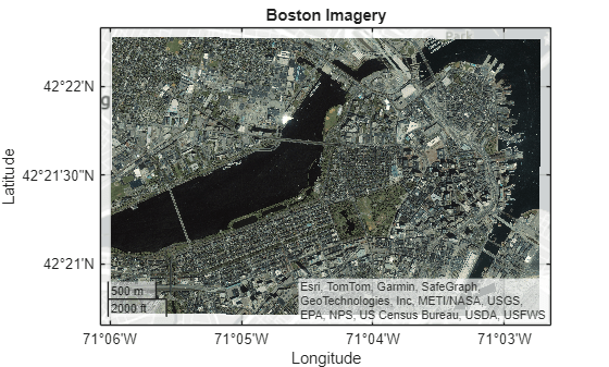
Apply a topographic basemap. Zoom out by changing the geographic limits.
geobasemap topographic
geolimits([42.3391 42.3756],[-71.1138 -71.0353])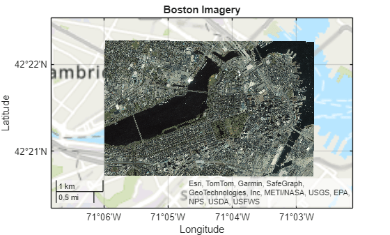
[1] The data used in this example includes material copyrighted by GeoEye, all rights reserved.
A grayscale image is a matrix with values that represent intensities within some range. For example, when the matrix is of type double, the intensities are in the range [0, 1].
Read elevation data for Colorado [1] into the workspace as a matrix and a raster reference object. Prepare to rescale the elevations by returning data of type double.
[Z,R] = readgeoraster("n39_w106_3arc_v2.dt1",OutputType="double");
Convert the elevation data to a grayscale image by rescaling the data to the interval [0, 1].
scaledZ = rescale(Z);
Create a map axes using the NAD83 / UTM Zone 13N projected CRS, which has the EPSG code 26913. Display the image on the map.
figure
pcrs = projcrs(26913);
newmap(pcrs)
geoimage(scaledZ,R)
Display an icon that represents Rocky Mountain National Airport in Colorado. Find the location of the airport by passing the street address to the geocode function.
GT = geocode("11755 Airport Way, Broomfield, CO 80021");
hold on
geoiconchart(GT.Shape.Latitude,GT.Shape.Longitude)
Add a title and subtitle.
title("Elevation Data as Grayscale Image")
subtitle(pcrs.Name)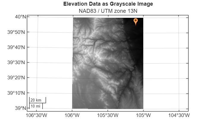
[1] The elevation data used in this example is from the US Geological Survey.
An indexed image is a matrix associated with a colormap. Each element of the indexed image maps to a row of the colormap, and each row of the colormap is an RGB triplet that specifies the red, green, and blue components of a color. To display an indexed image using the geoimage function, you must convert the indexed image to an RGB image.
Read land cover classification data for Oahu, Hawaii [1] into the workspace as a matrix, a raster reference object, and a colormap. Convert the indexed image to an RGB image by using the ind2rgb function.
[X,R,cmap] = readgeoraster("oahu_landcover.img");
RGB = ind2rgb(X,cmap);
Create a map axes using the projected CRS that is stored in the reference object. Display the RGB image on the map.
figure
pcrs = R.ProjectedCRS;
newmap(pcrs)
geoimage(RGB,R)
Add a title and subtitle.
title("Land Cover Classification")
subtitle(pcrs.ProjectionMethod)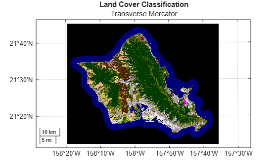
[1] The data used in this example is from the National Oceanic and Atmospheric Administration (NOAA).
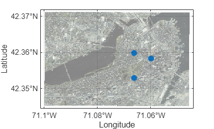
Display multiple images with coordinates in any supported geographic or projected CRS on the same map.
Read two images into the workspace as arrays and raster reference objects.
A low-resolution image of Boston [1] and the surrounding area. The metadata for the image,
boston_ovr.txt, indicates that the image is in geographic coordinates.A high-resolution image of a smaller area in Boston [1]. The metadata for the image,
boston_metadata.txt, indicates that the image is in projected coordinates.
low = imread("boston_ovr.jpg");
lowR = worldfileread("boston_ovr.jgw","geographic",size(low));

[high,highR] = readgeoraster("boston.tif");
View the CRS for the low-resolution image by querying the GeographicCRS property of the reference object. When the GeographicCRS property of the reference object is empty, the geoimage function assumes the geographic CRS based on the type of axes. For geographic axes, the function assumes the WGS84 CRS.
lowR.GeographicCRS
ans =

     []
View the CRS for the high-resolution image by querying the ProjectedCRS property of the reference object. To display images in projected coordinates using the geoimage function, the ProjectedCRS property of the reference object must not be empty.
highR.ProjectedCRS
ans =
  projcrs with properties:

                    Name: "NAD83 / Massachusetts Mainland"
           GeographicCRS: [1×1 geocrs]
        ProjectionMethod: "Lambert Conic Conformal (2SP)"
              LengthUnit: "U.S. survey foot"
    ProjectionParameters: [1×1 map.crs.ProjectionParameters]
Display the images on a geographic axes with no basemap.
figure
geobasemap none
geoimage(low,lowR)
hold on
geoimage(high,highR)
Create and display an area of interest (AOI) that represents the boundary of the high-resolution image. Then, zoom in to an area surrounding the high-resolution image.
aoi = aoiquad(highR);
geoplot(aoi,FaceColor="none",EdgeColor="w",LineWidth=1)

geolimits([42.3383 42.3747],[-71.1112 -71.0329])
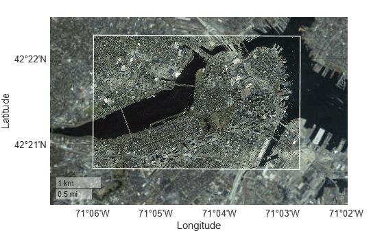
[1] The data used in this example includes material copyrighted by GeoEye, all rights reserved.
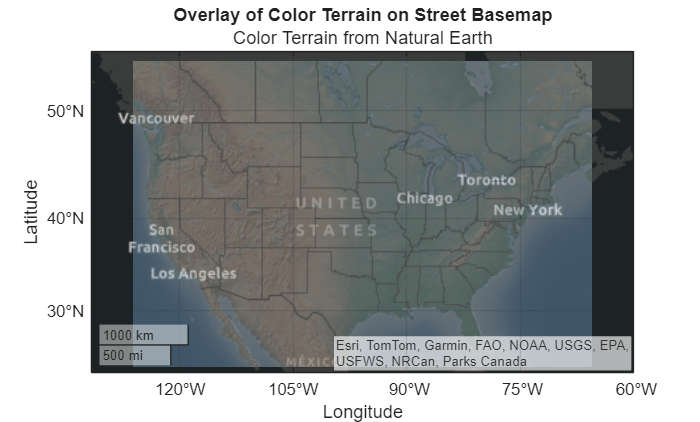
Read a basemap image for a region surrounding the conterminous US.
Create a geospatial table that contains an AOI by geocoding the placename United States (conterminous).
Buffer the AOI by 1 degree.
Get the latitude and longitude limits of the buffered AOI.
Read a basemap image using the latitude and longitude limits.
conus = geocode("United States (conterminous)");
buffered = buffer(conus.Shape,1);
[latlim,lonlim] = bounds(buffered);
[A,R] = readBasemapImage("colorterrain",latlim,lonlim,3);
Create a geographic axes that uses the streets-dark basemap. Then, display the basemap image as an overlay. To make the image semitransparent, specify the AlphaData argument as a scalar in the interval (0, 1).
figure
geobasemap streets-dark
geoimage(A,R,AlphaData=0.4)
Add a title and subtitle.
title("Overlay of Color Terrain on Street Basemap")
subtitle("Color Terrain from Natural Earth")
When an image contains a background, you can hide the background by changing the transparency of the corresponding image elements.
Read Image Data
Read land cover classification data for Oahu, Hawaii [1] into the workspace as a matrix, a raster reference object, and a colormap.
[X,R,cmap] = readgeoraster("oahu_landcover.img");Specify Transparency of Each Element
The metadata for the file, oahu_landcover.txt, indicates that the first row of the colormap corresponds to the background of the image.
Specify the transparency of each image element by creating a logical matrix. For image elements in the background, use 0, which is completely transparent. For the other elements, use 1, which is opaque.
imAlpha = (X ~= 0);
For indexed images, note that the value 0 maps to the first row of the colormap.
Display Image
Convert the indexed image to an RGB image. Then, display the image in a geographic axes with no basemap. Specify the transparency of the image using the AlphaData argument and the transparency matrix. Add a title and subtitle.
RGB = ind2rgb(X,cmap);

figure
geobasemap none
geoimage(RGB,R,AlphaData=imAlpha)
title("Land Cover Classification")
subtitle("No Background")
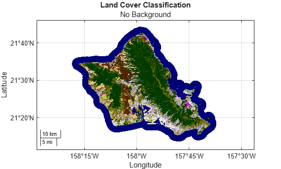
[1] The data used in this example is from the National Oceanic and Atmospheric Administration (NOAA).
By default, the geoimage function displays images on maps using bilinear interpolation. When the colors of your image represent distinct categories, or you want to see individual image elements in a highly zoomed-in view, use nearest-neighbor interpolation instead.
Read land cover classification data for Oahu, Hawaii [1] into the workspace as a matrix, a raster reference object, and a colormap. Convert the indexed image to an RGB image.
[X,R,cmap] = readgeoraster("oahu_landcover.img");
RGB = ind2rgb(X,cmap);
Create a map axes using the projected CRS that is stored in the reference object. Display the image using nearest-neighbor interpolation by specifying the Interpolation argument as "nearest".
figure
pcrs = R.ProjectedCRS;
newmap(pcrs)
geoimage(RGB,R,Interpolation="nearest");
Zoom in by using the geolimits function. Change the tick label format to decimal degrees. Add a title and subtitle.
geolimits([21.3746 21.4044],[-157.7371 -157.6885])
geotickformat -dd
title("Land Cover Classification")
subtitle("Using Nearest-Neighbor Interpolation")
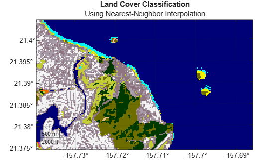
[1] The data used in this example is from the National Oceanic and Atmospheric Administration (NOAA).
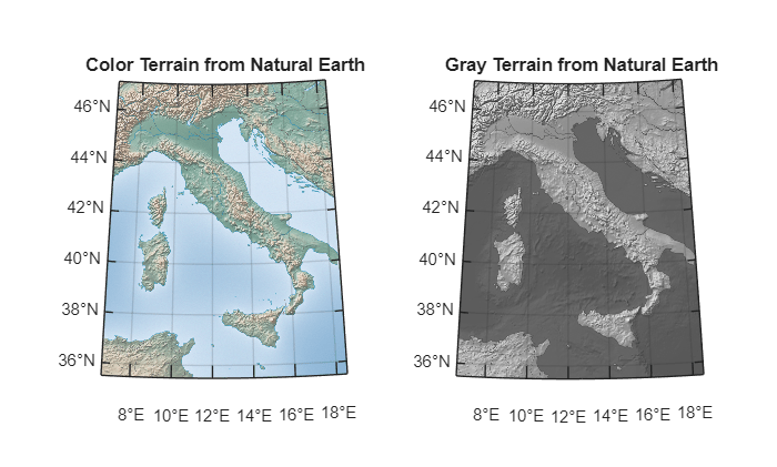
Create multiple maps in one figure by using a tiled chart layout.
Read two basemap images for a region surrounding Italy into the workspace as arrays and reference objects.
Create a geospatial table containing an AOI by geocoding the placename Italy.
Get the latitude and longitude limits of the AOI.
Read two basemaps images using the latitude and longitude limits.
italy = geocode("Italy");
[latlim,lonlim] = bounds(italy.Shape);
[colorA,colorR] = readBasemapImage("colorterrain",latlim,lonlim);
[grayA,grayR] = readBasemapImage("grayterrain",latlim,lonlim);
Create a projected CRS object that is appropriate for Italy. Use the RDN2008 / Italy zone (E-N) projected CRS, which has the EPSG code 7794.
pcrs = projcrs(7794);
Create a 1-by-2 tiled chart layout using the tiledlayout function.
figure
t = tiledlayout(1,2);
For each basemap image, place a map axes in a new tile. Display the basemap image, add a title, and apply a cartographic map layout. Change the cartographic limits to match the limits of the basemap image.
% Left tile
nexttile
mx1 = newmap(pcrs);
geoimage(mx1,colorA,colorR)
title(mx1,"Color Terrain from Natural Earth")
mx1.MapLayout="cartographic";
mx1.CartographicLatitudeLimits = latlim;
mx1.CartographicLongitudeLimits = lonlim;

% Right tile
nexttile
mx2 = newmap(pcrs);
geoimage(mx2,grayA,grayR)
title(mx2,"Gray Terrain from Natural Earth")
mx2.MapLayout = "cartographic";
mx2.CartographicLatitudeLimits = latlim;
mx2.CartographicLongitudeLimits = lonlim;
Read a GeoTIFF image of Boston [1] into the workspace as an m-by-n-by-3 array of RGB triplets and a raster reference object.
[A,R] = readgeoraster("boston.tif");Import a shapefile containing park data into the workspace as a geospatial table. The table represents the park using a polygon.
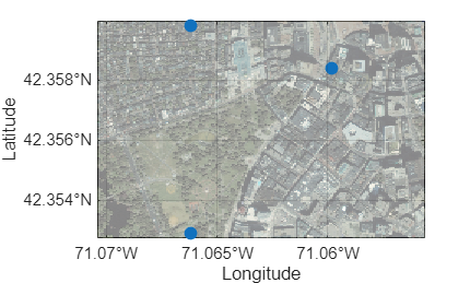
GT = readgeotable("bostonparks.shp");Display the image and the polygon on a geographic axes with no basemap. Prepare to change properties of the image by returning the Image object im.
figure
geobasemap none
im = geoimage(A,R);
hold on
geoplot(GT,FaceColor="w",EdgeColor="w")
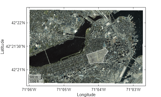
By default, MATLAB® includes both the image and the polygon in the automatic selection of the axes limits. Exclude the image from the automatic selection of limits by setting the AffectAutoLimits property to "off".
im.AffectAutoLimits = "off";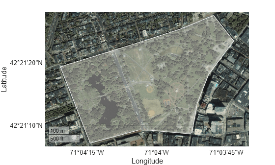
[1] The GeoTIFF file used in this example includes material copyrighted by GeoEye, all rights reserved.
Input Arguments
Name-Value Arguments
Specify optional pairs of arguments as
Name1=Value1,...,NameN=ValueN, where Name is
the argument name and Value is the corresponding value.
Name-value arguments must appear after other arguments, but the order of the
pairs does not matter.
Example:
geoimage(A,R,AlphaData=0.5) creates a semitransparent
image.
Note
Use name-value arguments to specify values for the properties of the
Image object created by this function. The properties listed here
are only a subset. For a full list, see Image Properties.
Transparency data, specified as one of these options:
A scalar — Use a consistent transparency across the entire image.
A matrix — Each element of the matrix specifies the transparency for the corresponding element of the image. The height and width of the matrix must match the height and width of
ColorData.
The interpretation of AlphaData depends on the data type:
If
AlphaDatais of typesingleordouble, then a value of0or less is completely transparent and a value of1or greater is opaque. Values between0and1are semitransparent.If
AlphaDatais an integer type, then the object uses the full range of data to determine the transparency. For example, ifAlphaDatais of typeint8, then-128is completely transparent and127is opaque. Values between-128and127are semitransparent.If
AlphaDatais of typelogical, then0is completely transparent and1is opaque.
Data Types: single | double | int8 | int16 | int32 | int64 | uint8 | uint16 | uint32 | uint64 | logical
Value indicating missing data, specified as one of these options:
A numeric scalar, when
ColorDatais a matrix.A 1-by-3 numeric vector, when
ColorDatais an m-by-n-by-3 array of RGB triplets.
When a matrix element or RGB triplet in ColorData matches the missing
data value, the corresponding element of the image appears transparent, regardless of the
value of AlphaData.
Interpolation method for displaying the image, specified as one of these options:
'bilinear'— Bilinear interpolation. Use this method to display an image with a smoother appearance. MATLAB® displays each image element by calculating a weighted average of the surrounding image elements.'nearest'— Nearest-neighbor interpolation. Use this method when the image has a small number of colors that represent distinct categories, or when you want to see individual image elements in a highly zoomed-in view. The value of a displayed image element is the value of the closest image element in theColorDataproperty of the image.
The value of Interpolation does not affect the data stored in the
ColorData or
AlphaData properties of the image.
Include the image in the automatic selection of the axes limits, specified as
"on" or "off", or as a logical
1 (true) or 0
(false). A value of "on" is equivalent to
true, and "off" is equivalent to
false. Thus, you can use the value of this property as a logical
value. The value is stored as an on/off logical value of type matlab.lang.OnOffSwitchState. The reference object associated with the
image defines the location of the image.
By default, the axes limits automatically change to include the data range for each successive
chart you create in the axes. Setting this property enables you to focus on the range of
a subset of data. To exclude the data range of an image from the automatic selection,
set its AffectAutoLimits property to
"off".
Image with AffectAutoLimits Set to "on"
| Image with AffectAutoLimits Set to "off"
|
|---|---|
|
|
Output Arguments
Tips
To display raster data using scaled colors and a colormap, use the
geopcolorfunction instead.If your image data is referenced to coordinate locations instead of a raster reference object, then you must convert the coordinates to a reference object before using the
geoimagefunction. For information about converting coordinates into reference objects, see Reference Regularly Spaced Raster Data Using Coordinates.
Version History
Introduced in R2026a
1 Alignment of boundaries and region labels are a presentation of the feature provided by the data vendors and do not imply endorsement by MathWorks®.