Estimate Transfer Function Models in the System Identification App

R2026b

Use the app to set model configuration and estimation options for estimating a transfer function model.

Prerequisites

• Import data into the System Identification app. See Represent Data. For supported data formats, see Data Supported by Transfer Function Models.

• Perform any required data preprocessing operations. If input and/or output signals contain nonzero offsets, consider detrending your data. See Data Preparation.

1. In the System Identification app, select Estimate > Transfer Function Models

   

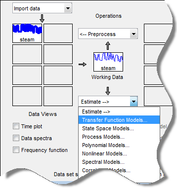
   The Transfer Functions dialog box opens.

   

   Tip

   For more information on the options in the dialog box, click Help.

2. In the Number of poles and Number of zeros fields, specify the number of poles and zeros of the transfer function as nonnegative integers.

   Multi-Input, Multi-Output Models

   For systems that are multiple input, multiple output, or both:

   • To use the same number of poles or zeros for all the input/output pairs, specify a scalar.

   • To use a different number of poles and zeros for the input/output pairs, specify an ny-by-nu matrix. ny is the number of outputs and nu is the number of inputs.

     Alternatively, click .

     

     The Transfer Function Orders dialog box opens where you specify the number of poles and zeros for each input/output pair, as well as whether to include feedthrough if you have specified your model as Discrete-time. Use the Output list to select an output.

     

3. Select Continuous-time or Discrete-time to specify whether the model is a continuous- or discrete-time transfer function.

   For discrete-time models, the number of poles and zeros refers to the roots of the numerator and denominator polynomials expressed in terms of the lag variable q^-1.

4. (For discrete-time models only) Specify whether to estimate the model feedthrough. Select the Feedthrough check box.

   

   A discrete-time model with 2 poles and 3 zeros takes the following form:

   $$H(z^{-1})=\frac{b0+b1z^{-1}+b2z^{-2}+b3z^{-3}}{1+a1z^{-1}+a2z^{-2}}$$

   When the model has direct feedthrough, b0 is a free parameter whose value is estimated along with the rest of the model parameters b1, b2, b3, a1, a2. When the model has no feedthrough, b0 is fixed to zero.

   Multi-Input, Multi-Output Models

   For models that are multi input, multi output or both, click Feedthrough.

   

   The Model Orders dialog box opens, where you specify to estimate the feedthrough for each input/output pair separately. Use the Output list to select an output.

   

5. Expand the Delay section to specify nominal values and constraints for transport delays for different input/output pairs.

   

   Use the Output list to select an output. Select the Fixed check box to specify a transport delay as a fixed value. Specify its nominal value in the Delay field.

6. Expand the Estimation Options section to specify estimation options.

   

   • Select Display progress to view the progress of the optimization.

   • Select Estimate covariance to estimate the covariance of the transfer function parameters.

   • (For frequency-domain data only) Specify whether to allow the estimation process to use parameter values that may lead to unstable models. Select the Allow unstable models option. An unstable model is delivered only if it produces a better fit to the data than other stable models computed during the estimation process.

   • Specify how to treat the initial conditions in the Initial condition list. For more information, see Specifying Initial Conditions for Iterative Estimation of Transfer Functions.

   • Expand Fit Frequency Range and set the range sliders to the desired passband to specify the frequency range over which the transfer function model must fit the data. By default the entire frequency range (0 to Nyquist frequency) is covered.

     

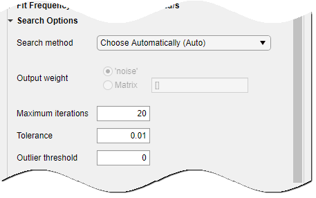
7. Expand Search Options to specify options for controlling the search iterations.

   

   Search Options

   In the Search Options section of Estimation Options, you can specify the following options:

   • Search method — Method used by the iterative search algorithm. Search method is auto by default. Search methods include Gauss-Newton(gn), Adaptive Gauss-Newton(gna), Levenberg-Marquardt(lm), Trust-Region Reflective Newton (lsqnonlin), Gradient Search (grad), Sequential Quadratic Programming (fmincon:sqp), or Interior Point (fmincon: interior-point). The descent direction is calculated successively at each iteration until a sufficient reduction in error is achieved.

     Output weight — Weighting applied to the loss function to be minimized. Use this option for multi-output estimations only. Specify as 'noise' or a positive semidefinite matrix of size equal the number of outputs.

   • Maximum iterations — Maximum number of iterations to use during search.

   • Tolerance — Tolerance value when the iterations should terminate.

   • Outlier threshold — Robustification of the quadratic criterion of fit.

8. Expand Regularization to obtain regularized estimates of model parameters. Specify the regularization constants Lambda and R.

   

   To learn more about regularization, see Regularized Estimates of Model Parameters.

9. Click Estimate to estimate the model. A new model gets added to the System Identification app.

Next Steps

• Validate the model by selecting the appropriate check box in the Model Views area of the System Identification app. For more information about validating models, see Validating Models After Estimation.

• Export the model to the MATLAB^® workspace for further analysis. Drag the model to the To Workspace rectangle in the System Identification app.