estimateStates
Description
estimates = estimateStates(filter,sensorData)insCF filter and the
sensor data. The function predicts the filter state estimates forward in time based on the
row times in sensorData and fuses data from each column of the table one-by-one along each row.
Examples
Estimate orientation from recorded IMU data by using a complementary filter, represented by an insCF filter object.
Load the rpy_9axis.mat file into the workspace. The file contains recorded accelerometer, gyroscope, and magnetometer sensor data from a device oscillating in pitch (around the y-axis), yaw (around the z-axis), and roll (around the x-axis). The file also contains the sample rate of the recording. Extract the sensor data and sample rate from the loaded workspace variable.
ld = load("rpy_9axis.mat");
accelerometerData = ld.sensorData.Acceleration;
gyroscopeData = ld.sensorData.AngularVelocity;
magnetometerData = ld.sensorData.MagneticField;
imuSampleRate = ld.Fs; % Hz
Create a timetable from the accelerometer, gyroscope, and magnetometer data.
imuDataTT = timetable(accelerometerData,gyroscopeData,magnetometerData,'SampleRate',imuSampleRate,'StartTime',seconds(1/imuSampleRate),'VariableNames',{'Accelerometer', 'Gyroscope', 'Magnetometer'});
Create an insCF filter object using sensor models for accelerometer, magnetometer, and gyroscope. To model orientation, specify insCFMotionOrientation as the motion model.
acc = insCFAccelerometer;
mag = insCFMagnetometer;
gyro = insCFGyroscope;
motionModel = insCFMotionOrientation;
filter = insCF(acc,mag,gyro,motionModel);
Specify the initial orientation of your sensors. You can obtain the initial orientation by using the ecompass function with the accelerometer and magnetometer data at the first time step.
initialOrientation = [0.006727036930852 -0.131203115007920 -0.058108427699335 -0.989628162602834];
stateparts(filter,"Orientation",initialOrientation)
Specify the sensor gains. The sensor gain value must be between 0 and 1.
gainparts(filter,"Accelerometer",0)
gainparts(filter,"Magnetometer",0.01)
Fuse the accelerometer, gyroscope, and magnetometer data using the insCF filter.
outTT = estimateStates(filter,imuDataTT);
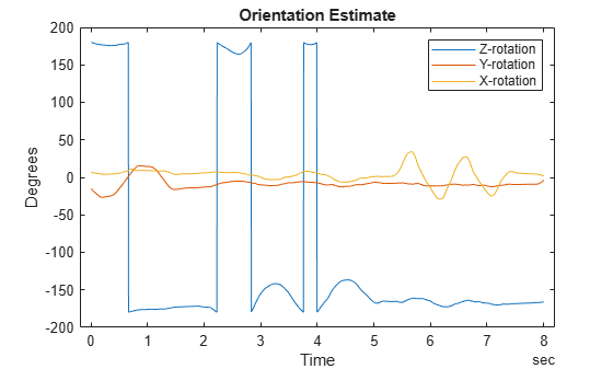
Visualize the estimated orientation.
t = outTT.Properties.RowTimes;
plot(t,eulerd(outTT.Orientation,"ZYX","frame"));
title("Orientation Estimate");
legend("Z-rotation","Y-rotation","X-rotation");
xlabel("Time");
ylabel("Degrees");
Estimate pose (orientation and position) and velocity from IMU and GPS data by using a complementary filter, represented by an insCF filter object.
Load the racetrackINSCFDataset.mat file, which contains a timetable with simulated accelerometer, gyroscope, magnetometer, and GPS sensor data for a racetrack-like trajectory, into the workspace. The file also contains the sample rate of the data.
load("raceTrackINSCFDataset.mat")Create an insCF filter object that includes the accelerometer, gyroscope, magnetometer, and GPS sensor objects, as well as an insCFMotionPose motion model object for modeling pose.
% Sensor object for predicting orientation
gyro = insCFGyroscope;
% Sensor objects for correcting orientation
accel = insCFAccelerometer;
mag = insCFMagnetometer;
% Sensor object for correcting position
gps = insCFGPS(ReferenceLocation=localOrigin);

% Pose motion model
motModel = insCFMotionPose;

% Filter object
filt = insCF(accel,mag,gyro,gps,motModel);
Specify the initial position, velocity, and orientation from the measurement data.
% Set initial position
stateparts(filt,"Position",initPos)
% Set initial orientation
stateparts(filt,"Orientation",initOrient)
% Set initial velocity
stateparts(filt,"Velocity",initVel)
Specify the sensor gains.
% Set Accelerometer gain
gainparts(filt,"Accelerometer",9.6335e-09)
% Set Magnetometer gain
gainparts(filt,"Magnetometer",0.01)
% Set GPS gain
gainparts(filt,"GPS",0.039246)
Fuse the sensor data using the filter. The filter estimates pose (orientation and position) and velocity. Extract the estimated position.
outTT = estimateStates(filt,sensorData);
estPos = outTT.Position;
Calculate the position RMS error.
posErr = truePos - estPos;
pRMS = sqrt(mean(posErr.^2));
fprintf("Position RMS Error:\tX: %.3f, Y: %.3f, Z: %.3f (meters) \n", pRMS(1),pRMS(2),pRMS(3))
Position RMS Error: X: 0.372, Y: 0.493, Z: 0.303 (meters)
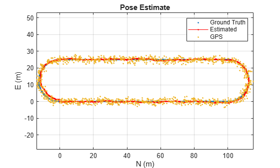
Visualize the estimated pose against the ground truth and GPS data.
figure
plot(truePos(:,1),truePos(:,2),".")
hold on
plot(estPos(:,1),estPos(:,2),"r.-")
gpsLocal = lla2ned(sensorData.GPS,localOrigin,"flat");
plot(gpsLocal(:,1),gpsLocal(:,2),".")

title("Pose Estimate")
legend("Ground Truth","Estimated","GPS")

grid on
xlabel("N (m)")
ylabel("E (m)")
axis equal
Input Arguments
Output Arguments
Extended Capabilities
Version History
Introduced in R2026a