initrpekf
Constant velocity range-parameterized EKF initialization
Syntax
Description
filter = initrpekf(detection)
The range-parameterized extended Kalman filter (RPEKF) is a Gaussian-sum filter (trackingGSF) with
multiple EKFs, each initialized at an estimated range of the target. Range-parameterization
is a commonly used technique to initialize a filter from an angle-only detection.
filter = initrpekf(detection,numFilters)
filter = initrpekf(detection,numFilters,rangeLimits)
Examples
The RPEKF is a special type of filter that can be initialized using angle-only measurements, that is, azimuth and/or elevation. When the 'Frame' is set to 'spherical' and 'HasRange' is set to 'false', the detection has [azimuth elevation] measurements. Specify the measurement parameters appropriately to define an angle-only measurement with no range information.
measParam = struct('Frame','spherical','HasRange',false,'OriginPosition',[100;10;0]);
The objectDetection class defines an interface to the angle-only detection measured by the sensor. The MeasurementParameters field of objectDetection carries information about what the sensor is measuring.
detection = objectDetection(0,[30;30],'MeasurementParameters',measParam,'MeasurementNoise',2*eye(2));
The initrpekf function uses the angle-only detection to initialize the RPEKF.
rpekf = initrpekf(detection) %#okrpekf =
trackingGSF with properties:
State: [6×1 double]
StateCovariance: [6×6 double]
TrackingFilters: {6×1 cell}
HasMeasurementWrapping: [1 1 1 1 1 1]
ModelProbabilities: [6×1 double]
MeasurementNoise: [2×2 double]
You can also initialize the RPEKF with 10 filters and to operate within the range limits of [1000, 10,000] scenario units.
rangeLimits = [1000 10000];
numFilters = 10;
rpekf = initrpekf(detection, numFilters, rangeLimits)
rpekf =
  trackingGSF with properties:

                     State: [6×1 double]
           StateCovariance: [6×6 double]

           TrackingFilters: {10×1 cell}
    HasMeasurementWrapping: [1 1 1 1 1 1 1 1 1 1]
        ModelProbabilities: [10×1 double]

          MeasurementNoise: [2×2 double]
You can also specify the initrpekf function as a FilterInitializationFcn to the trackerGNN object.
funcHandle = @(detection)initrpekf(detection,numFilters,rangeLimits)
funcHandle = function_handle with value:
    @(detection)initrpekf(detection,numFilters,rangeLimits)
tracker = trackerGNN('FilterInitializationFcn',funcHandle)tracker =
trackerGNN with properties:
TrackerIndex: 0
FilterInitializationFcn: @(detection)initrpekf(detection,numFilters,rangeLimits)
MaxNumTracks: 100
MaxNumDetections: Inf
MaxNumSensors: 20
Assignment: 'MatchPairs'
AssignmentThreshold: [30 Inf]
AssignmentClustering: 'off'
OOSMHandling: 'Terminate'
TrackLogic: 'History'
ConfirmationThreshold: [2 3]
DeletionThreshold: [5 5]
HasCostMatrixInput: false
HasDetectableTrackIDsInput: false
StateParameters: [1×1 struct]
ClassFusionMethod: 'None'
NumTracks: 0
NumConfirmedTracks: 0
EnableMemoryManagement: false
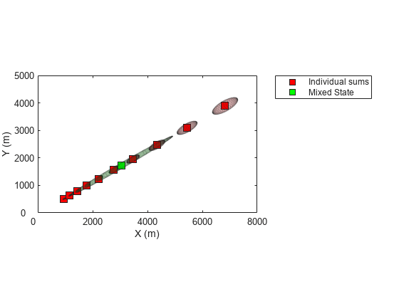
Visualize the filter.
tp = theaterPlot;
componentPlot = trackPlotter(tp,'DisplayName','Individual sums','MarkerFaceColor','r');
sumPlot = trackPlotter(tp,'DisplayName','Mixed State','MarkerFaceColor','g');

indFilters = rpekf.TrackingFilters;
pos = zeros(numFilters,3);
cov = zeros(3,3,numFilters);
for i = 1:numFilters
    pos(i,:) = indFilters{i}.State(1:2:end);
    cov(1:3,1:3,i) = indFilters{i}.StateCovariance(1:2:end,1:2:end);
end
componentPlot.plotTrack(pos,cov);

mixedPos = rpekf.State(1:2:end)';
mixedPosCov = rpekf.StateCovariance(1:2:end,1:2:end);
sumPlot.plotTrack(mixedPos,mixedPosCov);
Input Arguments
Output Arguments
References
[1] Peach, N. "Bearings-only tracking using a set of range-parameterised extended Kalman filters." IEE Proceedings-Control Theory and Applications 142, no. 1 (1995): 73-80.
Extended Capabilities
Version History
Introduced in R2018b