optByHestonFFT
Option price by Heston model using FFT and FRFT
Syntax
Description
[
computes vanilla European option price by Heston model, using Carr-Madan FFT and Chourdakis
FRFT methods.Price,StrikeOut] = optByHestonFFT(Rate,AssetPrice,Settle,Maturity,OptSpec,Strike,V0,ThetaV,Kappa,SigmaV,RhoSV)
Note
Alternatively, you can use the Vanilla object to price
vanilla options. For more information, see Get Started with Workflows Using Object-Based Framework for Pricing Financial Instruments.
[
adds optional name-value pair arguments. Price,StrikeOut] = optByHestonFFT(___,Name,Value)
Examples
Use optByHestonFFT to calibrate a FFT strike grid and then compute option prices and plot an option price surface.
Define Option Variables and Heston Model Parameters
AssetPrice = 80;
Rate = 0.03;
DividendYield = 0.02;
OptSpec = 'call';

V0 = 0.04;
ThetaV = 0.05;
Kappa = 1.0;
SigmaV = 0.2;
RhoSV = -0.7;
Compute the Option Prices for the Entire FFT (or FRFT) Strike Grid, Without Specifying "Strike"
Compute option prices and also output the corresponding strikes. If the Strike input is empty ( [] ), option prices will be computed on the entire FFT (or FRFT) strike grid. The FFT (or FRFT) strike grid is determined as exp(log-strike grid), where each column of the log-strike grid has NumFFT points with LogStrikeStep spacing that are roughly centered around each element of log(AssetPrice). The default value for NumFFT is 2^12. In addition to the prices in the first output, the optional last output contains the corresponding strikes.
Settle = datetime(2017,6,29);
Maturity = datemnth(Settle, 6);
Strike = []; % Strike is not specified (will use the entire FFT strike grid)

% Compute option prices for the entire FFT strike grid
[Call, Kout] =  optByHestonFFT(Rate, AssetPrice, Settle, Maturity, OptSpec, Strike, ...
    V0, ThetaV, Kappa, SigmaV, RhoSV, 'DividendYield', DividendYield);

% Show the lowest and highest strike values on the FFT strike grid
format
MinStrike = Kout(1) % Lowest possible strike in the current FFT strike grid
MinStrike =
2.9205e-135
MaxStrike = Kout(end) % Highest possible strike in the current FFT strike gridMaxStrike = 1.8798e+138
% Show a subset of the strikes and corresponding option prices
Range = (2046:2052);
[Kout(Range) Call(Range)]
ans = 7×2
50.4929 29.4843
58.8640 21.3767
68.6231 12.5614
80.0000 4.7008
93.2631 0.6496
108.7251 0.0144
126.7505 0.0001
Change the Number of FFT (or FRFT) Points, and Compare with optByHestonNI
Try a different number of FFT (or FRFT) points, and compare the results with direct numerical integration. Unlike optByHestonFFT, which uses FFT (or FRFT) techniques for fast computation across the whole range of strikes, the optByHestonNI function uses direct numerical integration and it is typically slower, especially for multiple strikes. However, the values computed by optByHestonNI can serve as a benchmark for adjusting the settings for optByHestonFFT.
% Try a smaller number of FFT (or FRFT) points
% (e.g. for faster performance or smaller memory footprint)
NumFFT = 2^10; % Smaller than the default value of 2^12
Strike = []; % Strike is not specified (will use the entire FFT strike grid)
[Call, Kout] = optByHestonFFT(Rate, AssetPrice, Settle, Maturity, OptSpec, Strike, ...
    V0, ThetaV, Kappa, SigmaV, RhoSV, 'DividendYield', DividendYield, 'NumFFT', NumFFT);

% Compare with numerical integration method
Range = (510:516);
Strike = Kout(Range);
CallFFT = Call(Range);
CallNI = optByHestonNI(Rate, AssetPrice, Settle, Maturity, OptSpec, Strike, V0, ...
    ThetaV, Kappa, SigmaV, RhoSV, 'DividendYield', DividendYield);
Error = abs(CallFFT-CallNI);
table(Strike, CallFFT, CallNI, Error)
ans=7×4 table
    Strike     CallFFT       CallNI         Error
    ______    _________    ___________    _________

    12.696       66.066         66.696      0.62964
    23.449       55.766         56.103      0.33672
    43.312       36.359         36.539      0.17974
        80       4.7727         4.7007     0.071928
    147.76     0.066156     2.3472e-08     0.066156
    272.93     0.013271    -2.5036e-09     0.013271
    504.11    0.0034504    -3.0876e-07    0.0034508
Make Further Adjustments to FFT (or FRFT)
If the values in the output CallFFT are significantly different from those in CallNI, try making adjustments to optByHestonFFT settings, such as CharacteristicFcnStep, LogStrikeStep, NumFFT, DampingFactor, and so on. Note that if (LogStrikeStep * CharacteristicFcnStep) is 2*pi/ NumFFT, FFT is used. Otherwise, FRFT is used.
Strike = []; % Strike is not specified (will use the entire FFT or FRFT strike grid)
[Call, Kout] = optByHestonFFT(Rate, AssetPrice, Settle, Maturity, OptSpec, Strike, ...
    V0, ThetaV, Kappa, SigmaV, RhoSV, 'DividendYield', DividendYield, ...
    'NumFFT', NumFFT, 'CharacteristicFcnStep', 0.065, 'LogStrikeStep', 0.001);

% Compare with numerical integration method
Strike = Kout(Range);
CallFFT = Call(Range);
CallNI = optByHestonNI(Rate, AssetPrice, Settle, Maturity, OptSpec, Strike, V0, ...
    ThetaV, Kappa, SigmaV, RhoSV, 'DividendYield', DividendYield);
Error = abs(CallFFT-CallNI);
table(Strike, CallFFT, CallNI, Error)
ans=7×4 table
    Strike    CallFFT    CallNI      Error
    ______    _______    ______    __________

    79.76      4.826      4.826    2.7708e-08
    79.84     4.7841     4.7841    3.0111e-08
    79.92     4.7423     4.7423    3.2376e-08
       80     4.7007     4.7007    3.4496e-08
    80.08     4.6593     4.6593    3.6457e-08
    80.16     4.6181     4.6181    3.8253e-08
    80.24      4.577      4.577    3.9872e-08
% Save the final FFT (or FRFT) strike grid for future reference. For
% example, it provides information about the range of Strike inputs for
% which the FFT (or FRFT) operation is valid.
FFTStrikeGrid = Kout;
MinStrike = FFTStrikeGrid(1) % Strike cannot be less than MinStrike
MinStrike =
47.9437
MaxStrike = FFTStrikeGrid(end) % Strike cannot be greater than MaxStrikeMaxStrike = 133.3566
Compute the Option Price for a Single Strike
Once the desired FFT (or FRFT) settings are determined, use the Strike input to specify the strikes rather than providing an empty array. If the specified strikes do not match a value on the FFT (or FRFT) strike grid, the outputs are interpolated on the specified strikes.
Settle = datetime(2017,6,29);
Maturity = datemnth(Settle, 6);
Strike = 80;

Call =  optByHestonFFT(Rate, AssetPrice, Settle, Maturity, OptSpec, Strike, ...
    V0, ThetaV, Kappa, SigmaV, RhoSV, 'DividendYield', DividendYield, 'NumFFT', NumFFT, ...
    'CharacteristicFcnStep', 0.065, 'LogStrikeStep', 0.001)
Call =
4.7007
Compute the Option Prices for a Vector of Strikes
Use the Strike input to specify the strikes.
Settle = datetime(2017,6,29);
Maturity = datemnth(Settle, 6);
Strike = (76:2:84)';

Call =  optByHestonFFT(Rate, AssetPrice, Settle, Maturity, OptSpec, Strike, ...
    V0, ThetaV, Kappa, SigmaV, RhoSV, 'DividendYield', DividendYield, 'NumFFT', NumFFT, ...
    'CharacteristicFcnStep', 0.065, 'LogStrikeStep', 0.001)
Call = 5×1

    7.0401
    5.8053
    4.7007
    3.7316
    2.8991
Compute the Option Prices for a Vector of Strikes and a Vector of Dates of the Same Lengths
Use the Strike input to specify the strikes. Also, the Maturity input can be a vector, but it must match the length of the Strike vector if the ExpandOutput name-value pair argument is not set to "true".
Settle = datetime(2017,6,29);
Maturity = datemnth(Settle, [12 18 24 30 36]); % Five maturities
Strike = [76 78 80 82 84]'; % Five strikes

Call =  optByHestonFFT(Rate, AssetPrice, Settle, Maturity, OptSpec, Strike, ...
    V0, ThetaV, Kappa, SigmaV, RhoSV, 'DividendYield', DividendYield, 'NumFFT', NumFFT, ...
    'CharacteristicFcnStep', 0.065, 'LogStrikeStep', 0.001) % Five values in vector output
Call = 5×1

    8.9560
    9.3419
    9.6240
    9.8560
   10.0500
Expand the Outputs for a Surface
Set the ExpandOutput name-value pair argument to "true" to expand the outputs into NStrikes-by NMaturities matrices. In this case, they are square matrices.
[Call, Kout] =  optByHestonFFT(Rate, AssetPrice, Settle, Maturity, OptSpec, Strike, ...
    V0, ThetaV, Kappa, SigmaV, RhoSV, 'DividendYield', DividendYield, 'NumFFT', NumFFT, ...
    'CharacteristicFcnStep', 0.065, 'LogStrikeStep', 0.001, ...
    'ExpandOutput', true) % (5 x 5) matrix outputs
Call = 5×5

    8.9560   10.4543   11.7058   12.8009   13.7728
    7.7946    9.3419   10.6337   11.7644   12.7685
    6.7244    8.3028    9.6240   10.7828   11.8134
    5.7475    7.3379    8.6771    9.8560   10.9074
    4.8645    6.4474    7.7930    8.9840   10.0500
Kout = 5×5

    76    76    76    76    76
    78    78    78    78    78
    80    80    80    80    80
    82    82    82    82    82
    84    84    84    84    84
Compute the Option Prices for a Vector of Strikes and a Vector of Dates of Different Lengths
When ExpandOutput is "true", NStrikes do not have to match NMaturities (that is, the output NStrikes-by-NMaturities matrix can be rectangular).
Settle = datetime(2017,6,29);
Maturity = datemnth(Settle, 12*(0.5:0.5:3)'); % Six maturities
Strike = (76:2:84)'; % Five strikes

Call =  optByHestonFFT(Rate, AssetPrice, Settle, Maturity, OptSpec, Strike, ...
    V0, ThetaV, Kappa, SigmaV, RhoSV, 'DividendYield', DividendYield, 'NumFFT', NumFFT, ...
    'CharacteristicFcnStep', 0.065, 'LogStrikeStep', 0.001, ...
    'ExpandOutput', true) % (5 x 6) matrix output
Call = 5×6

    7.0401    8.9560   10.4543   11.7058   12.8009   13.7728
    5.8053    7.7946    9.3419   10.6337   11.7644   12.7685
    4.7007    6.7244    8.3028    9.6240   10.7828   11.8134
    3.7316    5.7475    7.3379    8.6771    9.8560   10.9074
    2.8991    4.8645    6.4474    7.7930    8.9840   10.0500
Compute the Option Prices for a Vector of Strikes and a Vector of Asset Prices
When ExpandOutput is "true", the output can also be a NStrikes-by-NAssetPrices rectangular matrix by accepting a vector of asset prices.
Settle = datetime(2017,6,29);
Maturity = datemnth(Settle, 12); % Single maturity
ManyAssetPrices = [70 75 80 85]; % Four asset prices
Strike = (76:2:84)'; % Five strikes

Call =  optByHestonFFT(Rate, ManyAssetPrices, Settle, Maturity, OptSpec, Strike, ...
    V0, ThetaV, Kappa, SigmaV, RhoSV, 'DividendYield', DividendYield, 'NumFFT', NumFFT, ...
    'CharacteristicFcnStep', 0.065, 'LogStrikeStep', 0.001, ...
    'ExpandOutput', true) % (5 x 4) matrix output
Call = 5×4

    3.2944    5.8047    8.9560   12.6052
    2.6413    4.8810    7.7946   11.2507
    2.0864    4.0575    6.7244    9.9738
    1.6230    3.3325    5.7475    8.7783
    1.2429    2.7028    4.8645    7.6676
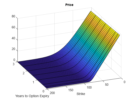
Plot an Option Price Surface
Use the Strike input to specify the strikes. Increase the value for NumFFT to support a wider range of strikes. Also, the Maturity input can be a vector. Set ExpandOutput to "true" to output the surface as a NStrikes-by-NMaturities matrix.
Settle = datetime(2017,6,29);
Maturity = datemnth(Settle, 12*[1/12 0.25 (0.5:0.5:3)]');
Times = yearfrac(Settle, Maturity);
Strike = (2:2:200)';

% Increase 'NumFFT' to support a wider range of strikes
NumFFT = 2^13;

Call =  optByHestonFFT(Rate, AssetPrice, Settle, Maturity, OptSpec, Strike, ...
    V0, ThetaV, Kappa, SigmaV, RhoSV, 'DividendYield', DividendYield, 'NumFFT', NumFFT, ...
    'CharacteristicFcnStep', 0.065, 'LogStrikeStep', 0.001, 'ExpandOutput', true);

[X,Y] = meshgrid(Times,Strike);

figure;
surf(X,Y,Call);
title('Price');
xlabel('Years to Option Expiry');
ylabel('Strike');
view(-112,34);
xlim([0 Times(end)]);
zlim([0 80]);
Input Arguments
Name-Value Arguments
Output Arguments
More About
References
[1] Albrecher, H., Mayer, P., Schoutens, W., and Tistaert, J. "The Little Heston Trap." Working Paper, Linz and Graz University of Technology, K.U. Leuven, ING Financial Markets, 2006.
[2] Carr, P. and D.B. Madan. “Option Valuation using the Fast Fourier Transform.” Journal of Computational Finance. Vol 2. No. 4. 1999.
[3] Chourdakis, K. “Option Pricing Using Fractional FFT.” Journal of Computational Finance. 2005.
[4] Heston, S. L. “A Closed-Form Solution for Options with Stochastic Volatility with Applications to Bond and Currency Options.” The Review of Financial Studies. Vol 6. No. 2. 1993.