RLS 적응 필터링을 사용한 적응 잡음 소거
이 예제에서는 RLS 필터를 사용하여 잡음이 있는 신호에서 유용한 정보를 추출하는 방법을 보여줍니다. 정보가 담긴 신호는 가산성 백색 가우스 잡음(AWGN)으로 인해 손상된 사인파입니다.
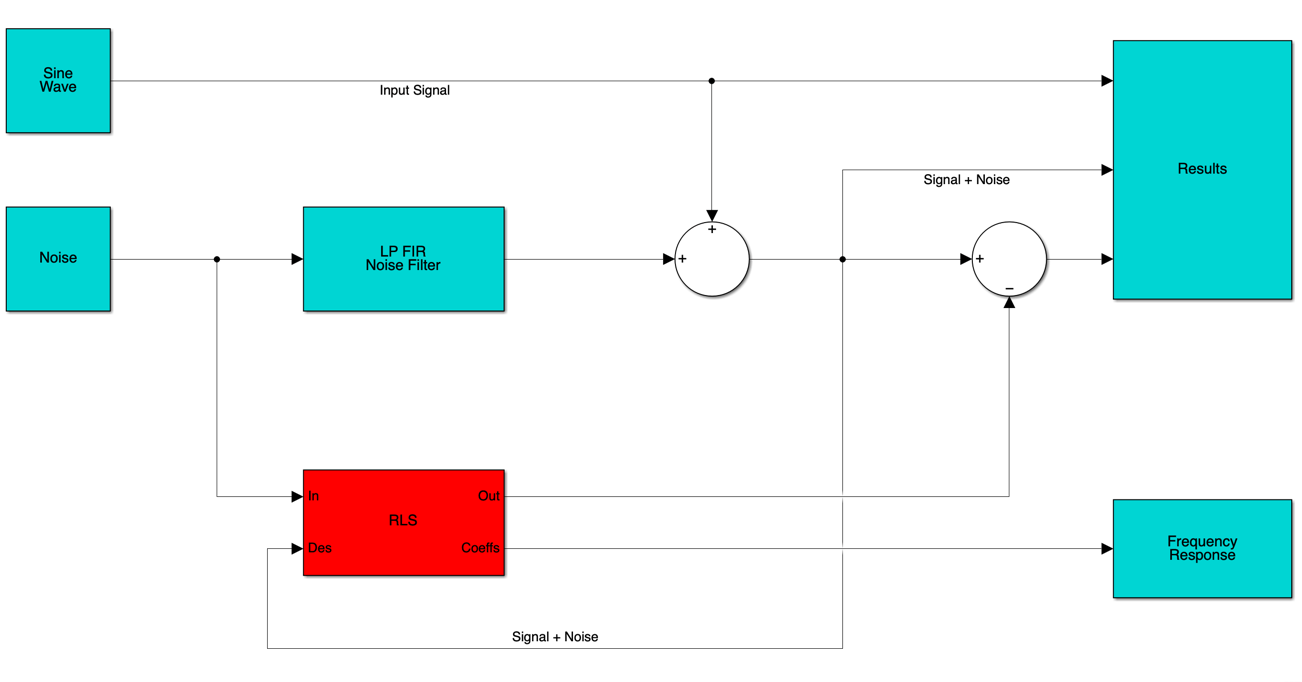
적응 잡음 소거 시스템은 두 개의 마이크를 사용한다고 가정합니다. 기본 마이크는 잡음이 있는 입력 신호를 포착하고, 보조 마이크는 정보가 담긴 신호와 상관관계가 없는 잡음이면서 기본 마이크가 포착하는 잡음과는 상관관계가 있는 잡음을 수신합니다.
참고: 이 예제는 제공된 Simulink® 모델 rlsdemo와 동일합니다.
이 모델은 적응 RLS 필터가 잡음이 있는 신호에서 유용한 정보를 추출하는 기능을 보여줍니다.
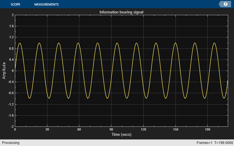
정보가 담긴 신호는 0.055 주기/샘플의 사인파입니다. 정보가 담긴 신호를 만들고 플로팅합니다.
signal = sin(2*pi*0.055*(0:1000-1)');
signalSource = dsp.SignalSource(signal,SamplesPerFrame=100,...
    SignalEndAction="Cyclic repetition");
scope = timescope(YLimits=[-2 2],Title="Information bearing signal")
scope =
  timescope handle with properties:

               SampleRate: 1
           TimeSpanSource: 'auto'
    TimeSpanOverrunAction: 'scroll'
              AxesScaling: 'manual'

  Show all properties
scope(signal(1:200));
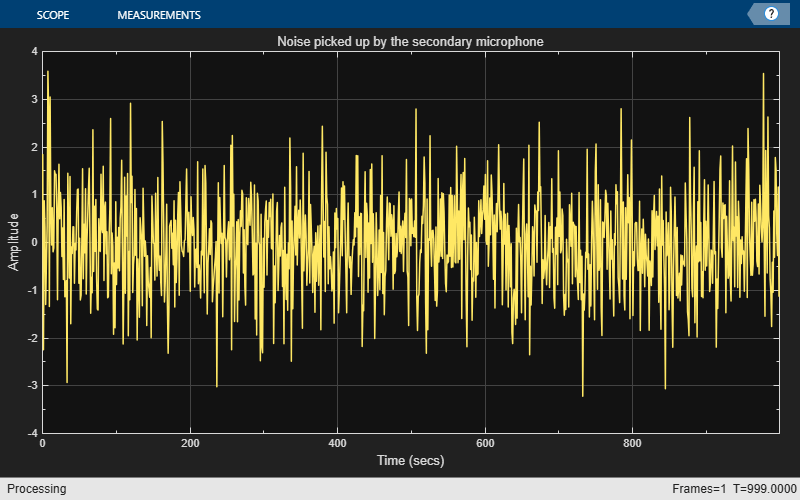
보조 마이크에서 포착한 잡음이 RLS 적응 필터에 대한 입력이 됩니다. 사인파를 손상시키는 잡음은 이 잡음에 저역통과 필터링을 적용한 잡음(이 잡음과 상관관계 있음)입니다. 적응 필터가 목표로 하는 신호는 이 필터링된 잡음과 정보가 담긴 신호를 합친 신호입니다. 잡음 신호를 만들고 플로팅합니다.
nvar  = 1.0;                  % Noise variance
noise = randn(1000,1)*nvar;   % White noise
noiseSource = dsp.SignalSource(noise,SamplesPerFrame=100,...
    SignalEndAction="Cyclic repetition");
scope = timescope(YLimits=[-4 4], Title="Noise picked up by the secondary microphone");
scope(noise);
정보가 담긴 신호를 손상시키는 잡음은 앞 단계에서 만든 잡음 신호를 필터링한 신호입니다. 잡음 신호에 작용하는 필터를 초기화합니다.
lp = dsp.FIRFilter('Numerator',fir1(31,0.5));% Low pass FIR filter
RLS 필터의 파라미터를 설정하고 필터를 초기화합니다.
M      = 32;                 % Filter order
delta  = 0.1;                % Initial input covariance estimate
P0     = (1/delta)*eye(M,M); % Initial setting for the P matrix
rlsfilt = dsp.RLSFilter(M,InitialInverseCovariance=P0);
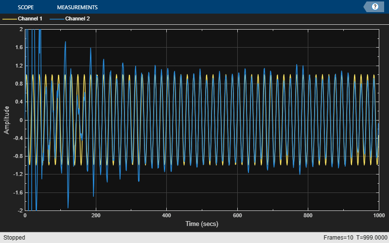
RLS 적응 필터를 1000회 반복해서 실행합니다. 적응 필터가 수렴함에 따라, 필터링된 잡음은 신호와 잡음의 합에서 완전히 차감되어야 합니다. 오차 e에는 원래 신호만 포함되어야 합니다.
scope = timescope(TimeSpan=1000,YLimits=[-2,2], ...
	              TimeSpanOverrunAction="scroll");
for k = 1:10
    n = noiseSource(); % Noise
    s = signalSource();
    d = lp(n) + s;
    [y,e]  = rlsfilt(n,d);
    scope([s,e]);
end
release(scope);
이 플롯은 FIR 필터의 응답에 적응 필터의 응답이 수렴하는 것을 보여줍니다.
visualizer = dsp.DynamicFilterVisualizer(64,NormalizedFrequency=true,...
    MagnitudeDisplay="Magnitude", ...
    FilterNames=["Adaptive Filter Response","Required Filter Response"]);
visualizer(rlsfilt.Coefficients,1,lp.Numerator,1);

참고 문헌
[1] S.Haykin, "Adaptive Filter Theory", 3rd Edition, Prentice Hall, N.J., 1996.