Time-Delay Approximation in Continuous-Time Closed-Loop Model

This example shows how to approximate delays in a continuous-time closed-loop system with internal delays, using pade.

Padé approximation is helpful when using analysis or design tools that do not support time delays.

1. Create sample continuous-time closed-loop system with an internal delay.

   

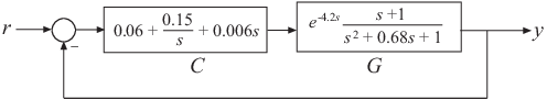
   Construct a model Tcl of the closed-loop transfer function from r to y.

   s = tf('s');
   G = (s+1)/(s^2+.68*s+1)*exp(-4.2*s);
   C = pid(0.06,0.15,0.006);
   Tcl = feedback(G*C,1);

   Examine the internal delay of Tcl.

   Tcl.InternalDelay

   ans = 4.2000
   

2. Compute the first-order Padé approximation of Tcl.

   Tnd1 = pade(Tcl,1);

   Tnd1 is a state-space (ss) model with no delays.

3. Compare the frequency response of the original and approximate models.

   h = bodeoptions;
   h.PhaseMatching = 'on';
   bodeplot(Tcl,'-b',Tnd1,'-.r',{.1,10},h);
   legend('Exact delay','First-Order Pade','Location','SouthWest');

   

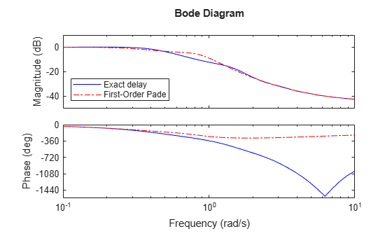
   The magnitude and phase approximation errors are significant beyond 1 rad/s.

4. Compare the time domain response of Tcl and Tnd1 using stepplot.

   stepplot(Tcl,'-b',Tnd1,'-.r');
   legend('Exact delay','First-Order Pade','Location','SouthEast');

   

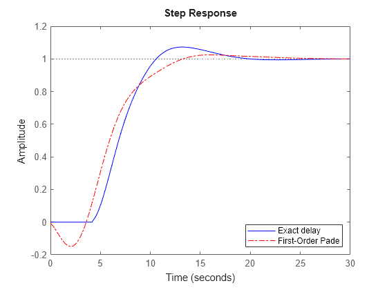
   Using the Padé approximation introduces a nonminimum phase artifact (“wrong way” effect) in the initial transient response.

5. Increase the Padé approximation order to see if this will extend the frequency with good phase and magnitude approximation.

   Tnd3 = pade(Tcl,3);

6. Observe the behavior of the third-order Padé approximation of Tcl. Compare the frequency response of Tcl and Tnd3.

   bodeplot(Tcl,'-b',Tnd3,'-.r',Tnd1,'--k',{.1,10},h);
   legend('Exact delay','Third-Order Pade','First-Order Pade',...
          'Location','SouthWest');

   

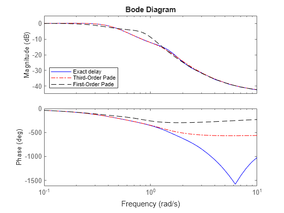
   The magnitude and phase approximation errors are reduced when a third-order Padé approximation is used.

Increasing the Padé approximation order extends the frequency band where the approximation is good. However, too high an approximation order may result in numerical issues and possibly unstable poles. Therefore, avoid Padé approximations with order N>10.