Approximate Model by Balanced Truncation at the Command Line
This example shows how to compute a reduced-order approximation of a model at the MATLAB® command line.
Balanced truncation removes the states with the lowest energy contribution to overall model behavior. Therefore, begin by examining the energy contribution of the model states. You choose the approximation order based on the number of states that make a significant contribution to the overall model behavior.
For this example, load a high-order model. hplant is a 23rd-order SISO model.
load ltiexamples hplant
order(hplant)
ans =
23
Create a model order reduction task using reducespec.
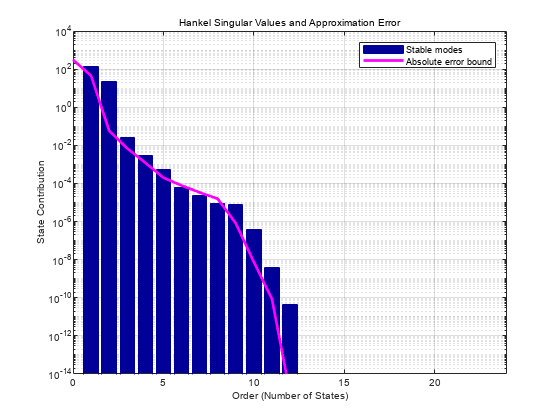
R = reducespec(hplant,"balanced");Examine the relative amount of energy per state in hplant using a Hankel singular-value (HSV) plot.
view(R)

Small Hankel singular values indicate that the associated states contribute little to the behavior of the system. The plot shows that two states account for most of the energy in the system. Therefore, try reducing the model to just first or second order using getrom.
hplant1 = getrom(R,Order=1,Method="Truncate");
hplant2 = getrom(R,Order=2,Method="Truncate");
The second argument to getrom specifies the target approximation order, so that hplant1 is a first-order approximation and hplant2 is a second-order approximation of hplant. By default, getrom discards the states with the smallest Hankel singular values, and alters the remaining states to preserve the DC gain of the system. Setting the Method option to "Truncate" causes getrom to discard low-energy states without altering the remaining states.
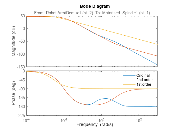
When working with reduced-order models, it is important to verify that the approximation does not introduce inaccuracies at frequencies that are important for your application. Therefore, compare the frequency responses of the original and approximated systems. For MIMO systems, use the sigmaplot command. For this SISO system, examine a Bode plot.
bodeplot(hplant,hplant2,hplant1)
legend('Original','2nd order','1st order')

The second-order approximation hplant2 matches the original 23rd-order system very well, especially at lower frequencies. The first-order system does not match as well.
In general, as you decrease the order of the approximated model, the frequency response of the approximated model begins to differ from the original model. Choose an approximation that is sufficiently accurate in the bands that are important to you. For example, in a control system you might want good accuracy inside the control bandwidth. Accuracy at frequencies far above the control bandwidth, where the gain rapidly rolls off, might be less important.
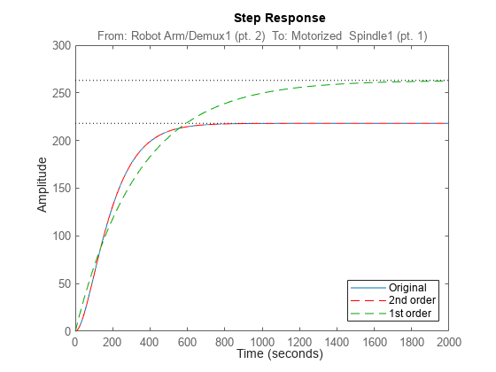
You can also validate the approximation in the time domain. For instance, examine the step responses of the original and reduced-order systems.
stepplot(hplant,hplant2,'r--',hplant1,'g--')
legend('Original','2nd order','1st order','Location','SouthEast')

This result confirms that the second-order approximation is a good match to the original 23rd-order system.