Compare Truncated and DC Matched Low-Order Model Approximations

This example shows how to compute a low-order approximation in two ways and compares the results. When you compute a low-order approximation by the balanced truncation method, you can either:

• Discard the states that make the smallest contribution to system behavior, altering the remaining states to preserve the DC gain of the system.

• Discard the low-energy states without altering the remaining states.

Which method you choose depends on what dynamics are most important to your application. In general, preserving DC gain comes at the expense of accuracy in higher-frequency dynamics. Conversely, state truncation can yield more accuracy in fast transients, at the expense of low-frequency accuracy.

This example compares the state-elimination methods of the balred command, Truncate and MatchDC. You can similarly control the state-elimination method in the Model Reducer app, on the Balanced Truncation tab, using the Preserve DC Gain check box, as shown.

Consider the following system.

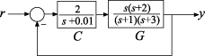
Create a closed-loop model of this system from r to y.

G = zpk([0 -2],[-1 -3],1);
C = tf(2,[1 1e-2]);
T = feedback(G*C,1)

T =
 
             2 s (s+2)
  --------------------------------
  (s+0.004277) (s+1.588) (s+4.418)
 
Continuous-time zero/pole/gain model.

T is a third-order system that has a pole-zero near-cancellation close to s = 0. Therefore, it is a good candidate for order reduction by approximation.

Compute two second-order approximations to T, one that preserves the DC gain and one that truncates the lowest-energy state without changing the other states. Use balredOptions to specify the approximation methods, MatchDC and Truncate, respectively.

matchopt = balredOptions('StateProjection','MatchDC');
truncopt = balredOptions('StateProjection','Truncate');
Tmatch = balred(T,2,matchopt);
Ttrunc = balred(T,2,truncopt);

Compare the frequency responses of the approximated models.

bodeplot(T,Tmatch,Ttrunc)
legend('Original','DC Match','Truncate')

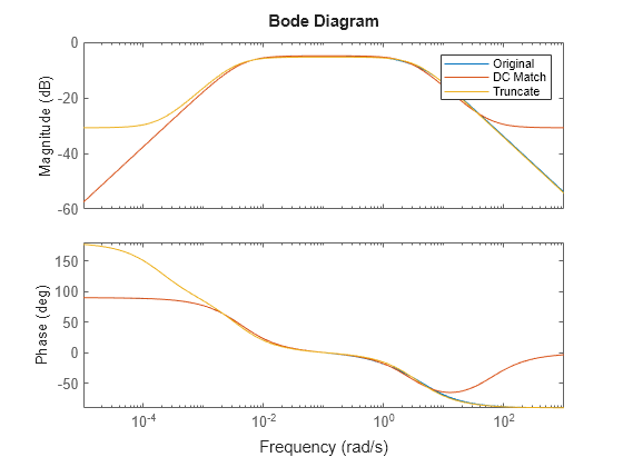
The truncated model Ttrunc matches the original model well at high frequencies, but differs considerably at low frequency. Conversely, Tmatch yields a good match at low frequencies as expected, at the expense of high-frequency accuracy.

You can also see the differences between the two methods by examining the time-domain response in different regimes. Compare the slow dynamics by looking at the step response of all three models with a long time horizon.

stepplot(T,Tmatch,'r--',Ttrunc,1500)
legend('Original','DC Match','Truncate')

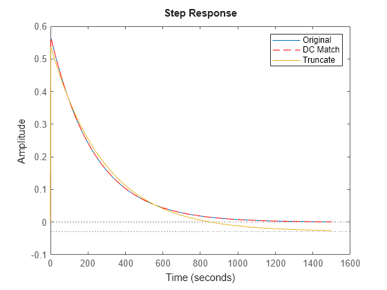
As expected, on long time scales the DC-matched approximation Tmatch has a very similar response to the original model.

Compare the fast transients in the step response.

stepplot(T,Tmatch,'r',Ttrunc,'g--',0.5)
legend('Original','DC Match','Truncate')

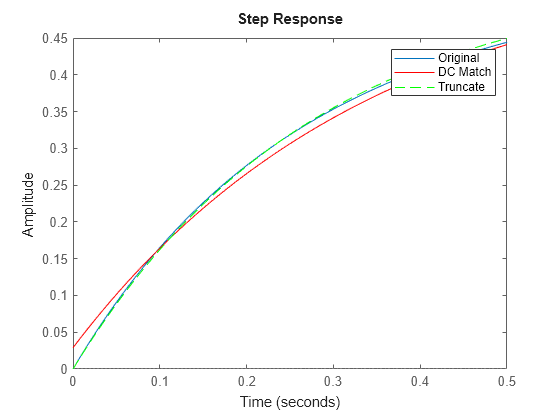
On short time scales, the truncated approximation Ttrunc provides a better match to the original model. Which approximation method you should use depends on which regime is most important for your application.