view

Plot state contributions when using proper orthogonal decomposition (POD) method

Since R2024b

Syntax

view(R,type)

view(R)

view(___,Parent=parent)

view(___,Name=Value)

hsvp = view(R,___)

view(R,"-help")

Description

Use view to graphically analyze the model and select a model order reduction criteria from a model order reduction task created using reducespec. For ProperOrthogonalDecomposition objects, you can visualize the state contributions as either principal singular values, normalized state energies, or neglected fraction of total energy. For the full workflow, see Task-Based Model Order Reduction Workflow.

view(R,type) creates a plot that helps you select the order of the reduced model. R specifies the model order reduction (MOR) specification object. Use the type argument to specify the plot type as either "sigma", "energy", or "loss".

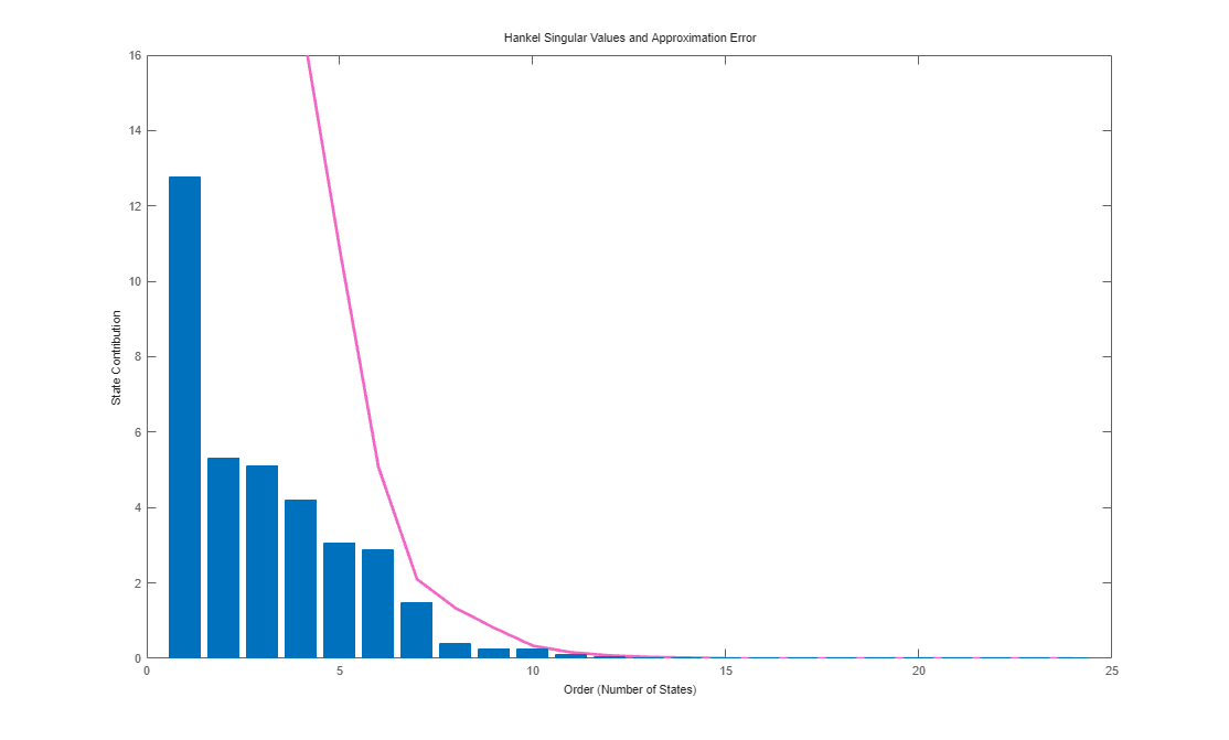
view(R) plots the default plot type for the model order reduction algorithm of R. For the POD method, this syntax plots principal singular values and associated error bounds.

view(___,Parent=parent) creates a plot in the specified parent graphics container, such as a Figure or TiledChartLayout. Use this syntax when you want to create a plot in a specified open figure or when creating apps in App Designer. You can specify the parent container after any of the input argument combinations in the previous syntaxes.

view(___,Name=Value) specifies additional options for customizing the appearance of Hankel singular value plots using one or more name-value arguments. For example, view(R,"sigma",YScale="Linear") plots the Hankel singular values using a linear scale for the y axis. For a list of available options, see hsvoptions.

hsvp = view(R,___) returns an HSVPlot object. To customize your plot, modify properties of the plot object using dot notation.

view(R,"-help") returns help specific to the MOR specification object R. The returned help shows plot types and syntaxes applicable to R.

Examples

Customize State Contribution Plots for POD

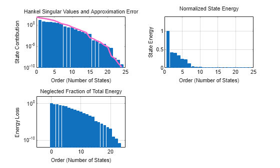
This example shows how to customize the state contribution plots obtained using the view function in the model order reduction workflow for POD method.

For this example, create a model order reduction specification for a LTI model. Generate a random discrete-time state-space model with 40 states.

rng(0)
sys = drss(40);

Create a specification object and compute the information.

R = reducespec(sys,"pod");
R = process(R);

Visualize the Hankel singular values.

view(R)

To customize the plot, you can use properties of the HSVPlot object as input arguments.

h = view(R,"sigma",YScale="linear");

Alternatively, you can set properties of the object directly using dot notation.

h.AxesStyle.GridVisible = "off";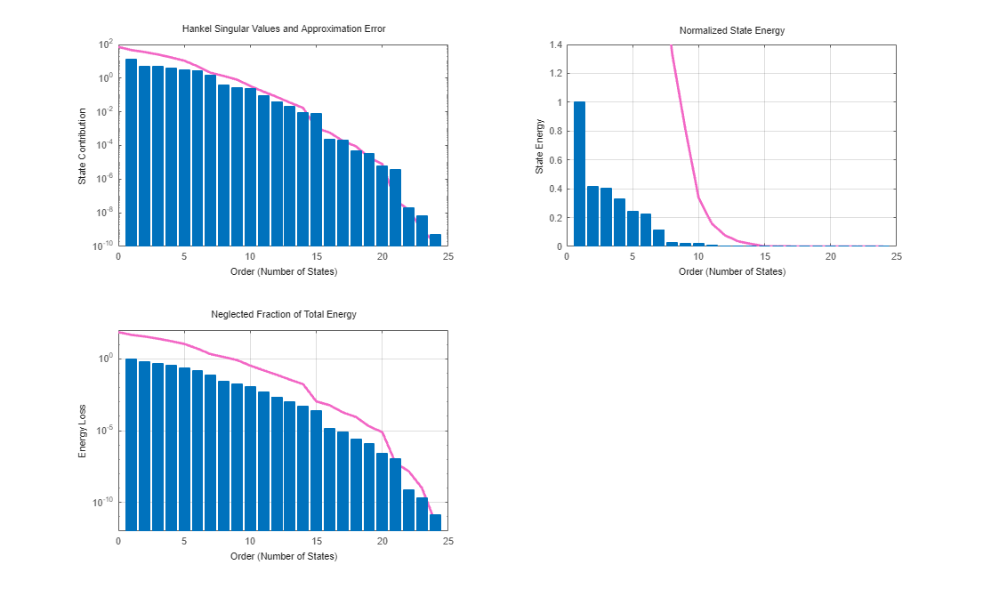

Additionally, you can visualize all plot types in the same figure using tiledlayout and customize them individually.

figure
tiledlayout("flow")
nexttile
view(R,Grid ="off")
nexttile
view(R,"energy",YScale="linear")
nexttile
view(R,"loss")

Input Arguments

R — Model order reduction specification object

ProperOrthogonalDecomposition object

Model order reduction specification object created using reducespec, specified as a ProperOrthogonalDecomposition object.

type — Plot type

"sigma" | "energy" | "loss"

Plot type, specified as one of these strings.

• "sigma" — Bar chart of Hankel singular values and associated error bounds.

• "energy" — Bar chart of normalized state energies.

• "loss" — Bar chart of neglected fraction of total energy.

If you do not specify this argument, the functions uses "sigma".

parent — Parent graphics container

Figure object | TiledChartLayout object | UIFigure object | UIGridLayout object | UIPanel object | UITab object | Axes object | UIAxes object

Parent graphics container, specified as one of these objects:

• Figure

• TiledChartLayout

• UIFigure

• UIGridLayout

• UIPanel

• UITab

You can also specify parent as an Axes or UIAxes object, which sets the plot parent to the parent of the specified axes object.

Output Arguments

hsvp — HSV plot object

HSVPlot object

HSV plot object, returned as an HSVPlot chart object. To customize the plot, modify the properties of hsvp using dot notation.

Version History

Introduced in R2024b

R2025a: Axes=AX input argument not recommended

Specifying the axes for plotting using Axes=AX is not recommended. Specify a parent graphics container using Parent=parent instead.

For example, the following code plots the response in an axes object obtained from a figure.

f = figure;
ax = gca;
view(R,Axes=ax)

To update the code, set the parent of the plot to the figure instead.

f = figure;
view(R,Parent=f)

R2025a: Specify parent graphics container

You can now plot state contributions in a parent graphics container, such as a Figure or TiledChartLayout object, using the parent argument.

Specifying parent as an Axes or UIAxes object sets the plot parent to the parent of the specified axes object.