qamdemod
직교위상 진폭 복조
설명
예제
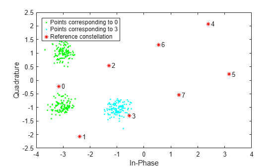
8-QAM 신호를 복조하고 심볼 0과 3에 대응되는 점을 플로팅합니다.
랜덤 8진 데이터 심볼을 생성합니다.
data = randi([0 7],1000,1);
8-QAM을 적용하여 data를 변조합니다.
txSig = qammod(data,8);
변조된 신호를 AWGN 채널에 통과시킵니다.
rxSig = awgn(txSig,18,'measured');초기 위상 /8을 사용하여 수신 신호를 복조합니다.
rxData = qamdemod(rxSig.*exp(-1i*pi/8),8);
기준 성상도 점을 생성합니다.
refpts = qammod((0:7)',8) .* exp(1i*pi/8);
심볼 0과 3에 대응되는 수신된 신호 점을 플로팅하고, 기준 성상도를 겹쳐 놓습니다. 그러한 심볼에 대응되는 수신된 데이터가 표시됩니다.
plot(rxSig(rxData==0),'g.');
hold on
plot(rxSig(rxData==3),'c.');
plot(refpts,'r*')
text(real(refpts)+0.1,imag(refpts),num2str((0:7)'))
xlabel('In-Phase')
ylabel('Quadrature')
legend('Points corresponding to 0','Points corresponding to 3', ...
    'Reference constellation','location','nw');
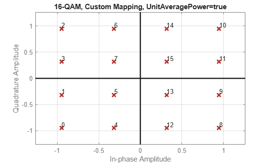
WLAN 심볼 매핑의 16-QAM을 사용하여 랜덤 데이터를 변조하고 복조합니다. 입력 데이터 심볼이 복조된 심볼과 일치하는지 확인합니다.
랜덤 심볼로 구성된 3차원 배열을 생성합니다.
x = randi([0,15],20,4,2);
WLAN 표준에 기반한 16-QAM 성상도의 사용자 지정 심볼 매핑을 만듭니다.
wlanSymMap = [2 3 1 0 6 7 5 4 14 15 13 12 10 11 9 8];
데이터를 변조하고 단위 평균 신호 전력을 갖도록 성상도를 설정합니다. 성상도를 플로팅합니다.
y = qammod(x,16,wlanSymMap, ...
    UnitAveragePower=true, ...
    PlotConstellation=true);
수신된 신호를 복조합니다.
z = qamdemod(y,16,wlanSymMap, ...
    UnitAveragePower=true);
복조된 신호가 원래 데이터와 동일한지 확인합니다.
isequal(x,z)
ans = logical
   1
고정소수점 QAM 신호를 복조하고 데이터가 올바르게 복구되는지 확인합니다.
변조 차수를 64로 설정하고 심볼당 비트 수를 결정합니다.
M = 64;
bitsPerSym = log2(M);
난수 비트를 생성합니다. 비트 모드에서 작업할 때 입력 데이터의 길이는 심볼당 비트 수의 정수 배수여야 합니다.
x = randi([0 1],10*bitsPerSym,1);
이진 심볼 매핑을 사용하여 입력 데이터를 변조합니다. 고정소수점 데이터를 출력하도록 변조기를 설정합니다. 숫자 데이터형은 16비트 워드 길이와 10비트 소수부 길이를 갖는 부호 있는 숫자입니다.
y = qammod(x,M,'bin', ...
    InputType='bit', ...
    OutputDataType=numerictype(1,16,10));
64-QAM 신호를 복조합니다. 복조된 데이터가 입력 데이터와 일치하는지 확인합니다.
z = qamdemod(y,M,'bin',OutputType='bit');
s = isequal(x,double(z))
s = logical
   1
AWGN에서 경판정 및 연판정 비터비 디코더의 비트 오류율(BER) 성능을 추정합니다. 이 성능을 코딩되지 않은 64-QAM 링크의 성능과 비교합니다.
시뮬레이션 파라미터를 설정합니다.
rng default
M = 64;                % Modulation order
k = log2(M);           % Bits per symbol
EbNoVec = (4:10)';     % Eb/No values (dB)
numSymPerFrame = 1000; % Number of QAM symbols per frame
BER 결과 벡터를 초기화합니다.
berEstSoft = zeros(size(EbNoVec));
berEstHard = zeros(size(EbNoVec));
비율 1/2, 제약 길이(constraint length) 7, 컨벌루션 코드로 트렐리스 구조체와 역추적 깊이를 설정합니다.
trellis = poly2trellis(7,[171 133]);
tbl = 32;
rate = 1/2;
주 처리 루프에서는 다음 단계를 수행합니다.
이진 데이터를 생성합니다.
데이터에 컨벌루션 인코딩을 수행합니다.
데이터 심볼에 QAM 변조를 적용합니다. 송신된 신호의 단위 평균 전력을 지정합니다.
변조된 신호를 AWGN 채널에 통과시킵니다.
경판정과 근사 LLR 방법을 사용하여 수신된 신호를 복조합니다. 수신된 신호의 단위 평균 전력을 지정합니다.
경판정과 비양자화 방법을 사용하여 신호에 비터비 디코딩을 수행합니다.
비트 오류 개수를 계산합니다.
while 루프는 100개의 오류가 발생하거나 비트가 송신될 때까지 데이터를 계속 처리합니다.
for n = 1:length(EbNoVec)
    % Convert Eb/No to SNR
    snrdB = EbNoVec(n) + 10*log10(k*rate);
    % Noise variance calculation for unity average signal power
    noiseVar = 10.^(-snrdB/10);
    % Reset the error and bit counters
    [numErrsSoft,numErrsHard,numBits] = deal(0);

    while numErrsSoft < 100 && numBits < 1e7
        % Generate binary data and convert to symbols
        dataIn = randi([0 1],numSymPerFrame*k,1);

        % Convolutionally encode the data
        dataEnc = convenc(dataIn,trellis);

        % QAM modulate
        txSig = qammod(dataEnc,M, ...
            InputType='bit', ...
            UnitAveragePower=true);

        % Pass through AWGN channel
        rxSig = awgn(txSig,snrdB,'measured');

        % Demodulate the noisy signal using hard decision (bit) and
        % soft decision (approximate LLR) approaches.
        rxDataHard = qamdemod(rxSig,M, ...
            OutputType='bit', ...
            UnitAveragePower=true);
        rxDataSoft = qamdemod(rxSig,M, ...
            OutputType='approxllr', ...
            UnitAveragePower=true, ...
            NoiseVariance=noiseVar);

        % Viterbi decode the demodulated data
        dataHard = vitdec(rxDataHard,trellis,tbl,'cont','hard');
        dataSoft = vitdec(rxDataSoft,trellis,tbl,'cont','unquant');

        % Calculate the number of bit errors in the frame.
        % Adjust for the decoding delay, which is equal to
        % the traceback depth.
        numErrsInFrameHard = ...
            biterr(dataIn(1:end-tbl),dataHard(tbl+1:end));
        numErrsInFrameSoft = ...
            biterr(dataIn(1:end-tbl),dataSoft(tbl+1:end));

        % Increment the error and bit counters
        numErrsHard = numErrsHard + numErrsInFrameHard;
        numErrsSoft = numErrsSoft + numErrsInFrameSoft;
        numBits = numBits + numSymPerFrame*k;

    end

    % Estimate the BER for both methods
    berEstSoft(n) = numErrsSoft/numBits;
    berEstHard(n) = numErrsHard/numBits;
end
추정된 하드 및 소프트 BER 데이터를 플로팅합니다. 코딩되지 않은 64-QAM 채널의 이론적 성능을 플로팅합니다.
semilogy(EbNoVec,[berEstSoft berEstHard],'-*')
hold on
semilogy(EbNoVec,berawgn(EbNoVec,'qam',M))
legend('Soft','Hard','Uncoded','location','best')
grid
xlabel('Eb/No (dB)')
ylabel('Bit Error Rate')
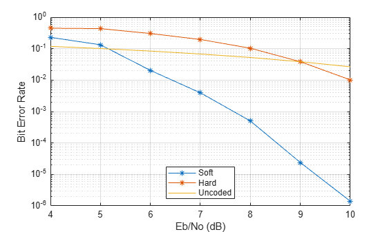
예상대로 연판정 디코딩이 최상의 결과를 생성합니다.
qamdemod 함수를 사용하여 OQPSK 변조 신호에 대한 연판정 출력값을 시뮬레이션합니다.
OQPSK 변조 신호를 생성합니다.
sps = 4;
msg = randi([0 1],1000,1);
oqpskMod = comm.OQPSKModulator( ...
    SamplesPerSymbol=sps, ...
    BitInput=true);
oqpskSig = oqpskMod(msg);
생성된 신호에 잡음을 추가합니다.
impairedSig = awgn(oqpskSig,15);
연판정 복조 수행하기
QPSK 등가 신호를 생성하여 동위상과 직교위상을 정렬합니다.
impairedQPSK = complex( ...
    real(impairedSig(1+sps/2:end-sps/2)), ...
    imag(impairedSig(sps+1:end)));
수신된 OQPSK 신호에 정합 필터링을 적용합니다.
halfSinePulse = sin(0:pi/sps:(sps)*pi/sps);
matchedFilter = dsp.FIRDecimator(sps,halfSinePulse, ...
    DecimationOffset=sps/2);
filteredQPSK = matchedFilter(impairedQPSK);
필터링된 OQPSK 신호에 소프트 복조를 수행하기 위해 qamdemod 함수를 사용합니다. qamdemod의 심볼 매핑을 comm.OQPSKModulator에서 사용한 심볼 매핑과 정렬한 다음 신호를 복조합니다.
oqpskModSymbolMapping = [1 3 0 2];
demodulated = qamdemod(filteredQPSK,4,oqpskModSymbolMapping, ...
    OutputType='llr');
qammod 함수와 qamdemod 함수를 사용할 때 helperAvgPow2MinD 유틸리티 함수를 사용하여 경판정 출력값에 대해 평균 전력 정규화를 적용합니다. 성상도를 정규화된 평균 전력으로 스케일링한 다음 기준 성상도와 스케일링된 성상도를 플로팅합니다.
지정된 평균 전력과 변조 차수를 기반으로 심볼의 최소 거리를 계산합니다.
M = 64;
avgPwr = 2;
minD = helperAvgPow2MinD(avgPwr,M);
[0, M- 1] 범위 내에 있는 임의의 정수로 구성된 신호를 변조하고, 변조된 심볼을 스케일링합니다.
x = randi([0,M-1],1000,1);
y = qammod(x,M);
yTx = (minD/2) .* y;
신호 평균 전력이 지정된 평균 전력 avgPow와 대략적으로 같음을 확인합니다.
sigPwr = mean(abs(yTx).^2)
sigPwr =
2.0141
avgPwr
avgPwr =
2
RF 또는 채널 손상을 적용하지 않은 상태로, 수신된 신호에 송신된 신호를 할당합니다. 수신된 신호를 왜곡할 손상이 없으므로 변조된 신호가 원본 신호와 일치합니다. 경판정을 사용하여 심볼을 복조하고 신호 복조가 올바른지 확인합니다.
yRx = yTx;
z = qamdemod(yRx*2/minD,M);
checkDemodIsEqual = isequal(x,z)
checkDemodIsEqual = logical
   1
refC = qammod([0:M-1]',M);
성상도를 표시합니다.
maxAx = ceil(max(abs(refC)));
cd = comm.ConstellationDiagram(2, ...
    'ShowReferenceConstellation',0, ...
    'ShowLegend',true, ...
    'XLimits',[-(maxAx) maxAx],'YLimits',[-(maxAx) maxAx], ...
    'ChannelNames', ...
    {'y','yTx'});
cd(y,yTx)

qammod 함수와 qamdemod 함수를 사용할 때 helperPeakPow2MinD 유틸리티 함수를 사용하여 경판정 출력값에 대해 피크 전력 정규화를 적용합니다. 성상도를 정규화된 피크 전력으로 스케일링한 다음 기준 성상도와 스케일링된 성상도를 플로팅합니다.
지정된 피크 전력과 변조 차수를 기반으로 심볼의 최소 거리를 계산합니다.
M = 16;
pkPwr = 30;
minD = helperPeakPow2MinD(pkPwr,M);
[0, M- 1] 범위 내에 있는 임의의 정수로 구성된 신호를 변조하고, 변조된 심볼을 스케일링합니다.
x = randi([0,M-1],1000,1);
y = qammod(x,M);
yTx = (minD/2) .* y;
신호 피크 전력이 지정된 피크 전력 pkPow와 대략적으로 같음을 확인합니다.
sigPwr = max(abs(yTx).^2)
sigPwr =
30
pkPwr
pkPwr =
30
RF 또는 채널 손상을 적용하지 않은 상태로, 수신된 신호에 송신된 신호를 할당합니다. 수신된 신호를 왜곡할 손상이 없으므로 변조된 신호가 원본 신호와 일치합니다. 경판정을 사용하여 심볼을 복조하고 신호 복조가 올바른지 확인합니다.
yRx = yTx;
z = qamdemod(yRx*2/minD,M);
checkDemodIsEqual = isequal(x,z)
checkDemodIsEqual = logical
   1
refC = qammod([0:M-1]',M);
성상도를 표시합니다.
maxAx = ceil(max(abs(refC)));
cd = comm.ConstellationDiagram(2, ...
    'ShowReferenceConstellation',0, ...
    'ShowLegend',true, ...
    'XLimits',[-(maxAx) maxAx],'YLimits',[-(maxAx) maxAx], ...
    'ChannelNames', ...
    {'y','yTx'});
cd(y,yTx)

대규모 데이터 세트로 작업할 때, GPU를 사용하면 통신 시스템 시뮬레이션 속도를 크게 높일 수 있습니다. MATLAB®에서 GPU 가속의 실용적인 이점과 고려 사항을 보여주기 위해, 이 워크플로는 CPU 플랫폼과 GPU 플랫폼에서의 시뮬레이션 실행 시간을 비교하여 사용자가 MATLAB에서 GPU 가속의 실용적인 이점과 고려 사항을 이해하도록 돕습니다.
먼저, runQAMDemodulator 헬퍼 함수를 사용하여 기준을 설정합니다. 이 함수는 여러 프레임과 두 개의 공간 채널에 걸쳐 수신된 1e6개의 심볼에 대해 비트별 근사 LLR을 계산하여, 현실적인 채널 조건을 시뮬레이션합니다. 그런 다음 AMD EPYC 7262 8‑Core Processor(CPU)에서 timeit를 사용하여 실행 시간을 벤치마킹합니다. 아래 코드는 prototype 변수를 사용하여 계산 타깃을 제어하고, 시뮬레이션을 함수 핸들로 래핑한 다음 실행 시간을 측정하여 결과를 표시합니다.
CPU에서 시뮬레이션 시간을 벤치마킹합니다.
prototype = 0;
f = @()runQAMDemodulator(prototype);
tCPU = timeit(f,1);
disp("Simulation time on a CPU: "+tCPU+"s")
Simulation time on a CPU: 0.091397s
다음으로, prototype을 gpuArray로 변환하여 GPU에서 동일한 벤치마크를 실행합니다. 이 예제에서는 NVIDIA RTX A5000을 사용합니다.
prototype = gpuArray(prototype);
f = @()runQAMDemodulator(prototype);
tGPU = gputimeit(f,1);
disp("Simulation time on a GPU: "+tGPU+"s")
Simulation time on a GPU: 0.0488s
마지막으로, CPU와 비교하여 GPU를 사용하여 달성한 속도 향상을 계산하고 표시합니다.
disp("Simulation speedup on GPU vs CPU: "+tCPU/tGPU)Simulation speedup on GPU vs CPU: 1.8729
GPU에서의 시뮬레이션이 CPU보다 1.87배 빠릅니다.
CPU와 GPU 모두에서 엔드 투 엔드 통신 시스템 시뮬레이션의 실행 시간을 벤치마킹합니다. runSimulation 헬퍼 함수를 사용하여 대규모 데이터 배치를 엔드 투 엔드로 처리합니다. 먼저 CPU에서 시뮬레이션을 실행하고 GPU에서 다시 실행한 다음, 실행 시간과 속도 향상을 보고합니다.
CPU에서 데이터를 처리합니다.
prototype = 0;
f = @()runSimulation(prototype);
tCPU = timeit(f,1);
disp("System simulation time on a CPU: "+tCPU+"s")
System simulation time on a CPU: 0.35853s
GPU에서 데이터를 처리합니다.
prototype = gpuArray(prototype);
f = @()runSimulation(prototype);
tGPU = gputimeit(f,1);
disp("System simulation time on a GPU: "+tGPU+"s")
System simulation time on a GPU: 0.083089s
시스템 수준 시뮬레이션 속도 향상을 보고합니다.
disp("System simulation speedup on GPU vs CPU: "+tCPU/tGPU)System simulation speedup on GPU vs CPU: 4.3151
GPU에서의 시뮬레이션이 CPU보다 4.3배 빠릅니다.
헬퍼 함수
runQAMDemodulator 헬퍼 함수를 사용하여 CPU와 GPU의 기준을 확인합니다.
function demodOut = runQAMDemodulator(prototype)
    M = 256;    % 256-QAM
    nVar = 0.2;
    for k=1:5
        rxSig = rand(100e3, 2, like=cast(1i, like=prototype));
        demodOut = qamdemod(rxSig, M, UnitAveragePower=true, OutputType="approxllr", NoiseVariance=nVar);
    end
end
runSimulation 헬퍼 함수를 사용하여 CPU와 GPU 모두에서 엔드 투 엔드 통신 시스템 시뮬레이션의 실행 시간을 벤치마킹합니다.
function bitErr = runSimulation(prototype)
    M = 256;    % 256-QAM
    snrDB = 10; % SNR, in dB
    nBits = log2(M);
    ber = comm.ErrorRate();

    for k=1:5
        m = randi([0,1], nBits*100e3, 2, like=prototype);
        txSig = qammod(m, M, UnitAveragePower=true, InputType="bit");
        [rxSig, nVar] = awgn(txSig, snrDB);
        b = qamdemod(rxSig, M, UnitAveragePower=true, OutputType="approxllr", NoiseVariance=nVar);
        bitErr = ber(b(:)<0, m(:));
    end
end