Working with GEO Series Data
This example shows how to retrieve gene expression data series (GSE) from the NCBI Gene Expression Omnibus (GEO) and perform basic analysis on the expression profiles.
Introduction
The NCBI Gene Expression Omnibus (GEO) is the largest public repository of high-throughput microarray experimental data. GEO data have four entity types including GEO Platform (GPL), GEO Sample (GSM), GEO Series (GSE) and curated GEO DataSet (GDS).
A Platform record describes the list of elements on the array in the experiment (e.g., cDNAs, oligonucleotide probesets). Each Platform record is assigned a unique and stable GEO accession number (GPLxxx).
A Sample record describes the conditions under which an individual Sample was handled, the manipulations it underwent, and the abundance measurement of each element derived from it. Each Sample record is assigned a unique and stable GEO accession number (GSMxxx).
A Series record defines a group of related Samples and provides a focal point and description of the whole study. Series records may also contain tables describing extracted data, summary conclusions, or analyses. Each Series record is assigned a unique GEO accession number (GSExxx).
A DataSet record (GDSxxx) represents a curated collection of biologically and statistically comparable GEO Samples. GEO DataSets (GDSxxx) are curated sets of GEO Sample data.
More information about GEO can be found in GEO Overview. Bioinformatics Toolbox™ provides functions that can retrieve and parse GEO format data files. GSE, GSM, GSD and GPL data can be retrieved by using the getgeodata function. The getgeodata function can also save the retrieved data in a text file. GEO Series records are available in SOFT format files and in tab-delimited text format files. The function geoseriesread reads the GEO Series text format file. The geosoftread function reads the usually quite large SOFT format files.
In this example, you will retrieve the GSE5847 data set from GEO database, and perform statistical testing on the data. GEO Series GSE5847 contains experimental data from a gene expression study of tumor stroma and epithelium cells from 15 inflammatory breast cancer (IBC) cases and 35 non-inflammatory breast cancer cases (Boersma et al. 2008).
Retrieving GEO Series Data
The function getgeodata returns a structure containing data retrieved from the GEO database. You can also save the returned data in its original format to your local file system for use in subsequent MATLAB® sessions. Note that data in public repositories is frequently curated and updated; therefore the results of this example might be slightly different when you use up-to-date datasets.
gseData = getgeodata('GSE5847', 'ToFile', 'GSE5847.txt')Use the geoseriesread function to parse the previously downloaded GSE text format file.
gseData = geoseriesread('GSE5847.txt')
gseData =

  struct with fields:

    Header: [1×1 struct]
      Data: [22283×95 bioma.data.DataMatrix]
The structure returned contains a Header field that stores the metadata of the Series data, and a Data field that stores the Series matrix data.
Exploring GSE Data
The GSE5847 matrix data in the Data field are stored as a DataMatrix object. A DataMatrix object is a data structure like MATLAB 2-D array, but with additional metadata of row names and column names. The properties of a DataMatrix can be accessed like other MATLAB objects.
get(gseData.Data)
            Name: ''
        RowNames: {22283×1 cell}
        ColNames: {1×95 cell}
           NRows: 22283
           NCols: 95
           NDims: 2
    ElementClass: 'double'
The row names are the identifiers of the probe sets on the array; the column names are the GEO Sample accession numbers.
gseData.Data(1:5, 1:5)
ans =

                 GSM136326    GSM136327    GSM136328    GSM136329    GSM136330
    1007_s_at     10.45       9.3995       9.4248       9.4729       9.2788
    1053_at      5.7195       4.8493       4.7321       4.7289       5.3264
    117_at       5.9387       6.0833        6.448       6.1769       6.5446
    121_at       8.0231       7.8947        8.345       8.1632       8.2338
    1255_g_at    3.9548       3.9632       3.9641       4.0878       3.9989
The Series metadata are stored in the Header field. The structure contains Series information in the Header.Series field, and sample information in the Header.Sample field.
gseData.Header
ans =

  struct with fields:

     Series: [1×1 struct]
    Samples: [1×1 struct]
The Series field contains the title of the experiment and the microarray GEO Platform ID.
gseData.Header.Series
ans =

  struct with fields:

                         title: 'Tumor and stroma from breast by LCM'
                 geo_accession: 'GSE5847'
                        status: 'Public on Sep 30 2007'
               submission_date: 'Sep 15 2006'
              last_update_date: 'Nov 14 2012'
                     pubmed_id: '17999412'
                       summary: 'Tumor epithelium and surrounding stromal cells were isolated using laser capture microdissection of human breast cancer to examine differences in gene expression based on tissue types from inflammatory and non-inflammatory breast cancer↵Keywords: LCM'
                overall_design: 'We applied LCM to obtain samples enriched in tumor epithelium and stroma from 15 IBC and 35 non-IBC cases to study the relative contribution of each component to the IBC phenotype and to patient survival. '
                          type: 'Expression profiling by array'
                   contributor: 'Stefan,,Ambs↵Brenda,,Boersma↵Mark,,Reimers'
                     sample_id: 'GSM136326 GSM136327 GSM136328 GSM136329 GSM136330 GSM136331 GSM136332 GSM136333 GSM136334 GSM136335 GSM136336 GSM136337 GSM136338 GSM136339 GSM136340 GSM136341 GSM136342 GSM136343 GSM136344 GSM136345 GSM136346 GSM136347 GSM136348 GSM136349 GSM136350 GSM136351 GSM136352 GSM136353 GSM136354 GSM136355 GSM136356 GSM136357 GSM136358 GSM136359 GSM136360 GSM136361 GSM136362 GSM136363 GSM136364 GSM136365 GSM136366 GSM136367 GSM136368 GSM136369 GSM136370 GSM136371 GSM136372 GSM136373 GSM136374 GSM136375 GSM136376 GSM136377 GSM136378 GSM136379 GSM136380 GSM136381 GSM136382 GSM136383 GSM136384 GSM136385 GSM136386 GSM136387 GSM136388 GSM136389 GSM136390 GSM136391 GSM136392 GSM136393 GSM136394 GSM136395 GSM136396 GSM136397 GSM136398 GSM136399 GSM136400 GSM136401 GSM136402 GSM136403 GSM136404 GSM136405 GSM136406 GSM136407 GSM136408 GSM136409 GSM136410 GSM136411 GSM136412 GSM136413 GSM136414 GSM136415 GSM136416 GSM136417 GSM136418 GSM136419 GSM136420 '
                  contact_name: 'Stefan,,Ambs'
            contact_laboratory: 'LHC'
             contact_institute: 'NCI'
               contact_address: '37 Convent Dr Bldg 37 Room 3050'
                  contact_city: 'Bethesda'
                 contact_state: 'MD'
    contact_zip0x2Fpostal_code: '20892'
               contact_country: 'USA'
            supplementary_file: 'ftp://ftp.ncbi.nlm.nih.gov/pub/geo/DATA/supplementary/series/GSE5847/GSE5847_RAW.tar'
                   platform_id: 'GPL96'
                platform_taxid: '9606'
                  sample_taxid: '9606'
                      relation: 'BioProject: http://www.ncbi.nlm.nih.gov/bioproject/97251'
gseData.Header.Samples
ans =

  struct with fields:

                         title: {1×95 cell}
                 geo_accession: {1×95 cell}
                        status: {1×95 cell}
               submission_date: {1×95 cell}
              last_update_date: {1×95 cell}
                          type: {1×95 cell}
                 channel_count: {1×95 cell}
               source_name_ch1: {1×95 cell}
                  organism_ch1: {1×95 cell}
           characteristics_ch1: {2×95 cell}
                  molecule_ch1: {1×95 cell}
          extract_protocol_ch1: {1×95 cell}
                     label_ch1: {1×95 cell}
            label_protocol_ch1: {1×95 cell}
                     taxid_ch1: {1×95 cell}
                  hyb_protocol: {1×95 cell}
                 scan_protocol: {1×95 cell}
                   description: {1×95 cell}
               data_processing: {1×95 cell}
                   platform_id: {1×95 cell}
                  contact_name: {1×95 cell}
            contact_laboratory: {1×95 cell}
             contact_institute: {1×95 cell}
               contact_address: {1×95 cell}
                  contact_city: {1×95 cell}
                 contact_state: {1×95 cell}
    contact_zip0x2Fpostal_code: {1×95 cell}
               contact_country: {1×95 cell}
            supplementary_file: {1×95 cell}
                data_row_count: {1×95 cell}
The data_processing field contains the information of the preprocessing methods, in this case the Robust Multi-array Average (RMA) procedure.
gseData.Header.Samples.data_processing(1)
ans =

  1×1 cell array

    {'RMA'}
The source_name_ch1 field contains the sample source:
sampleSources = unique(gseData.Header.Samples.source_name_ch1);
sampleSources{:}
ans =

    'human breast cancer stroma'


ans =

    'human breast cancer tumor epithelium'
The field Header.Samples.characteristics_ch1 contains the characteristics of the samples.
gseData.Header.Samples.characteristics_ch1(:,1)
ans =

  2×1 cell array

    {'IBC'     }
    {'Deceased'}
Determine the IBC and non-IBC labels for the samples from the Header.Samples.characteristics_ch1 field as group labels.
sampleGrp = gseData.Header.Samples.characteristics_ch1(1,:);
Retrieving GEO Platform (GPL) Data
The Series metadata told us the array platform id: GPL96, which is an Affymetrix® GeneChip® Human Genome U133 array set HG-U133A. Retrieve the GPL96 SOFT format file from GEO using the getgeodata function. For example, assume you used the getgeodata function to retrieve the GPL96 Platform file and saved it to a file, such as GPL96.txt. Use the geosoftread function to parse this SOFT format file.
gplData = geosoftread('GPL96.txt')
gplData =

  struct with fields:

                 Scope: 'PLATFORM'
             Accession: 'GPL96'
                Header: [1×1 struct]
    ColumnDescriptions: {16×1 cell}
           ColumnNames: {16×1 cell}
                  Data: {22283×16 cell}
The ColumnNames field of the gplData structure contains names of the columns for the data:
gplData.ColumnNames
ans =

  16×1 cell array

    {'ID'                              }
    {'GB_ACC'                          }
    {'SPOT_ID'                         }
    {'Species Scientific Name'         }
    {'Annotation Date'                 }
    {'Sequence Type'                   }
    {'Sequence Source'                 }
    {'Target Description'              }
    {'Representative Public ID'        }
    {'Gene Title'                      }
    {'Gene Symbol'                     }
    {'ENTREZ_GENE_ID'                  }
    {'RefSeq Transcript ID'            }
    {'Gene Ontology Biological Process'}
    {'Gene Ontology Cellular Component'}
    {'Gene Ontology Molecular Function'}
You can get the probe set ids and gene symbols for the probe sets of platform GPL69.
gplProbesetIDs = gplData.Data(:, strcmp(gplData.ColumnNames, 'ID'));
geneSymbols = gplData.Data(:, strcmp(gplData.ColumnNames, 'Gene Symbol'));
Use gene symbols to label the genes in the DataMatrix object gseData.Data. Be aware that the probe set IDs from the platform file may not be in the same order as in gseData.Data. In this example they are in the same order.
Change the row names of the expression data to gene symbols.
gseData.Data = rownames(gseData.Data, ':', geneSymbols);
Display the first five rows and five columns of the expression data with row names as gene symbols.
gseData.Data(1:5, 1:5)
ans =

              GSM136326    GSM136327    GSM136328    GSM136329    GSM136330
    DDR1       10.45       9.3995       9.4248       9.4729       9.2788
    RFC2      5.7195       4.8493       4.7321       4.7289       5.3264
    HSPA6     5.9387       6.0833        6.448       6.1769       6.5446
    PAX8      8.0231       7.8947        8.345       8.1632       8.2338
    GUCA1A    3.9548       3.9632       3.9641       4.0878       3.9989
Analyzing the Data
Bioinformatics Toolbox and Statistics and Machine Learning Toolbox™ offer a wide spectrum of analysis and visualization tools for microarray data analysis. However, because it is not our main goal to explain the analysis methods in this example, you will apply only a few of the functions to the gene expression profile from stromal cells. For more elaborate examples about feature selection tools available, see Select Features for Classifying High-Dimensional Data.
The experiment was performed on IBC and non-IBC samples derived from stromal cells and epithelial cells. In this example, you will work with the gene expression profile from stromal cells. Determine the sample indices for the stromal cell type from the gseData.Header.Samples.source_name_ch1 field.
stromaIdx = strcmpi(sampleSources{1}, gseData.Header.Samples.source_name_ch1);
Determine number of samples from stromal cells.
nStroma = sum(stromaIdx)
nStroma =

    47
stromaData = gseData.Data(:, stromaIdx);
stromaGrp = sampleGrp(stromaIdx);
Determine the number of IBC and non-IBC stromal cell samples.
nStromaIBC = sum(strcmp('IBC', stromaGrp))
nStromaIBC =

    13
nStromaNonIBC = sum(strcmp('non-IBC', stromaGrp))
nStromaNonIBC =

    34
You can also label the columns in stromaData with the group labels:
stromaData = colnames(stromaData, ':', stromaGrp);
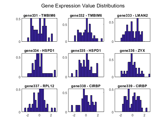
Display the histogram of the normalized gene expression measurements of a specified gene. The x-axes represent the normalized expression level. For example, inspect the distribution of the gene expression values of these genes.
fID = 331:339;
zValues = zscore(stromaData.(':')(':'), 0, 2);
bw = 0.25;
edges = -10:bw:10;
bins = edges(1:end-1) + diff(edges)/2;
histStroma = histc(zValues(fID, :)', edges) ./ (stromaData.NCols*bw);
figure;
for i = 1:length(fID)
    subplot(3,3,i);
    bar(edges, histStroma(:,i), 'histc')
    xlim([-3 3])
    if i <= length(fID)-3
        ax = gca;
        ax.XTickLabel = [];
    end
    title(sprintf('gene%d - %s', fID(i), stromaData.RowNames{fID(i)}))
end
sgtitle('Gene Expression Value Distributions')

The gene expression profile was accessed using the Affymetrix GeneChip more than 22,000 features on a small number of samples (~100). Among the 47 tumor stromal samples, there are 13 IBC and 34 non-IBC. But not all the genes are differentially expressed between IBC and non-IBC tumors. Statistical tests are needed to identify a gene expression signature that distinguish IBC from non-IBC stromal samples.
Use genevarfilter to filter out genes with a small variance across samples.
[mask, stromaData] = genevarfilter(stromaData);
stromaData.NRows
ans =

       20055
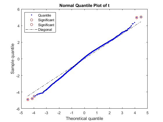
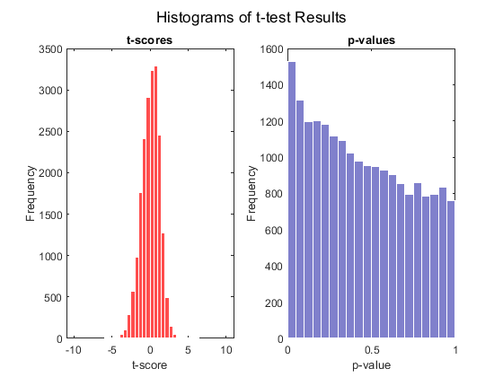
Apply a t-statistic on each gene and compare p-values for each gene to find significantly differentially expressed genes between IBC and non-IBC groups by permuting the samples (1,000 times for this example).
rng default
[pvalues, tscores] = mattest(stromaData(:, 'IBC'), stromaData(:, 'non-IBC'),...
                           'Showhist', true', 'showplot', true, 'permute', 1000);


Select the genes at a specified p-value.
sum(pvalues < 0.001)
ans =

    52
There are about 50 genes selected directly at p-values < 0.001.
Sort and list the top 20 genes:
testResults = [pvalues, tscores];
testResults = sortrows(testResults);
testResults(1:20, :)
ans =

                        p-values      t-scores
    INPP5E              2.3318e-05     5.0389
    ARFRP1 /// IGLJ3    2.7575e-05     4.9753
    USP46               3.4336e-05    -4.9054
    GOLGB1              4.7706e-05    -4.7928
    TTC3                0.00010695    -4.5053
    THUMPD1             0.00013164    -4.4317
                        0.00016042     4.3656
    MAGED2              0.00017042    -4.3444
    DNAJB9               0.0001782    -4.3266
    KIF1C               0.00022122     4.2504
                        0.00022237    -4.2482
    DZIP3               0.00022414    -4.2454
    COPB1               0.00023199    -4.2332
    PSD3                0.00024649    -4.2138
    PLEKHA4             0.00026505      4.186
    DNAJB9               0.0002767    -4.1708
    CNPY2                0.0002801    -4.1672
    USP9X               0.00028442    -4.1619
    SEC22B              0.00030146    -4.1392
    GFER                0.00030506    -4.1352
References
[1] Boersma, B.J., Reimers, M., Yi, M., Ludwig, J.A., et al. "A stromal gene signature associated with inflammatory breast cancer", International Journal of Cancer, 122(6):1324-32, 2008.