Import Measured Field Data and Visualize Radiation Pattern
This example shows how to visualize a radiation pattern and vector fields from the imported pattern data. Use the patternCustom function to plot the field data in 3D. This function also allows you to view the sliced data. Alternatively, use the polarpattern object to visualize the field data in 2D polar format. The polarpattern function allows you to interact with the data and perform antenna specific measurements. You can also plot the vector fields at a point in space using the fieldsCustom function.
Import Field Data
Use the readmatrix function to import the field data stored in a .csv file. In the first part of this example, you use the patternCustom function to visualize the data in 3D. You can also use this function to visualize 2D slices of the 3D pattern.
M = readmatrix("CustomPattern_testfile.csv");Plot 3D Radiation Pattern Using Polar Coordinate System
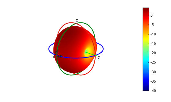
Specify the electric field magnitude (MagE) vector/matrix along with the theta and phi vectors to plot the 3D radiation pattern. The patternCustom function uses polar coordinate system by default. If MagE is a matrix, it must be of size phi-by-theta. If MagE is a vector, then all the 3 arguments MagE, phi and theta must be of the same size.
patternCustom(M(:,3),M(:,2),M(:,1));
Plot 3D Radiation Pattern Using Rectangular Coordinate System
Specify the CoordinateSystem argument as "rectangular" to plot the 3D radiation pattern using a rectangular coordinate system.
patternCustom(M(:,3),M(:,2),M(:,1),CoordinateSystem="rectangular");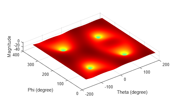
Visualize 2D Slices of 3D Pattern
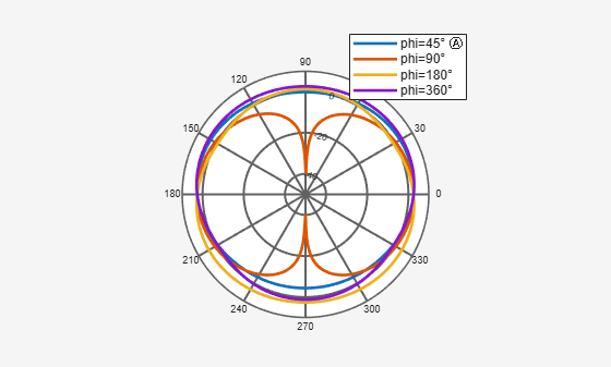
Specify the CoordinateSystem argument as "polar" to plot a 2D slice using a polar coordinate system plot. Specify the Slice argument to either "phi" or "theta", depending on the plane you want to view the data in. Additionally, specify the SliceValue argument as a vector of phi or theta angles for the slices as input values.
patternCustom(M(:,3),M(:,2),M(:,1),CoordinateSystem="polar",...
    Slice="phi",SliceValue=[45 90 180 360]);
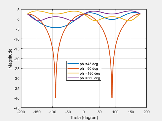
Specify the CoordinateSystem argument as "rectangular" to plot the same data using the rectangular coordinate system.
patternCustom(M(:,3),M(:,2),M(:,1),CoordinateSystem="rectangular",...
     Slice="phi",SliceValue=[45 90 180 360]);
Plot 2D Polar Data
Use the polarpattern function to plot pattern data in polar format as shown below. The generated plot is interactive and allows you to perform antenna specific measurements. The data for this illustration is stored in a MAT file which stores directivity values calculated over 360 degrees with one degree separation.
load polardata
p = polarpattern(ang, D);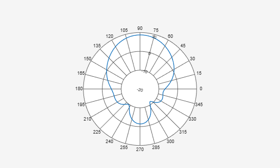
Right-click inside the figure window to interact with the plot. The figure below shows a screen shot of the context menu. Context menus can be used to do measurements such as peak detection, beamwidth calculation etc. You can also add a cursor by right clicking inside the polar circle.
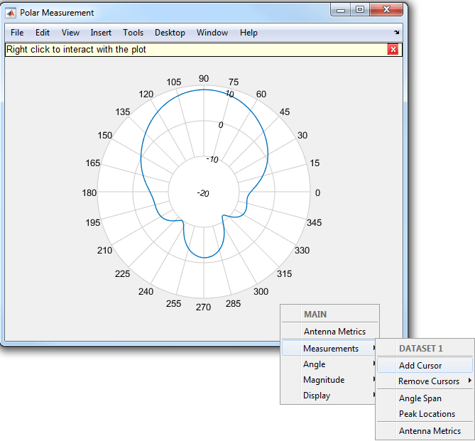
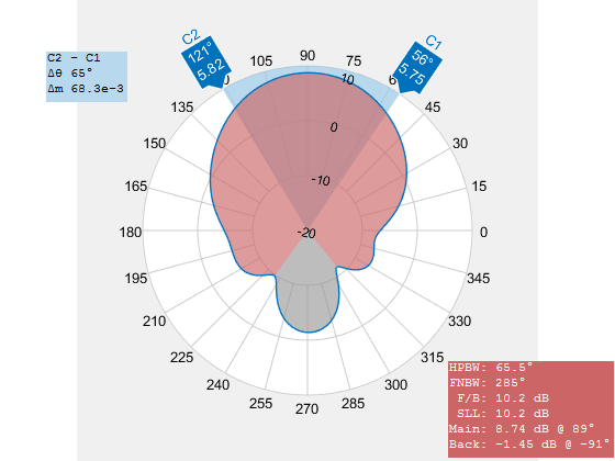
Select the Antenna Metrics option in the context menu shown above, to visualize the antenna specific measurements as shown below.
Plot Vector Field at Point in Space
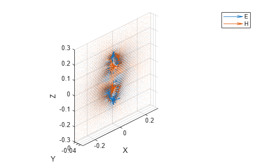
Use the fieldsCustom function to plot vector electric and/or magnetic fields at any point in space as shown below. The MAT file EHfielddata contains the E and H field data at the points in space specified by the x, y and z coordinates. The electric and magnetic fields are complex quantities and have x, y and z components at every point in space. The fields can be artificially scaled for better visualization.
load EHfielddata;
figure
fieldsCustom(H,points,5);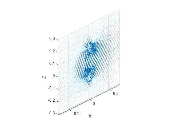
The function is used to plot one field quantity at a time. To plot both E and H fields on the same plot, use the hold on command.
figure
fieldsCustom(gca,E,points,5);
hold on;
fieldsCustom(gca,H,points,5);
hold off;
legend("E","H");