NR Positioning Using PRS
This example shows how to calculate the position of user equipment (UE) within a network of gNodeBs (gNBs) by using an NR positioning reference signal (PRS). The example uses the observed time difference of arrival (OTDOA) positioning approach to estimate the UE position in 2-D, relative to (0,0).
Introduction
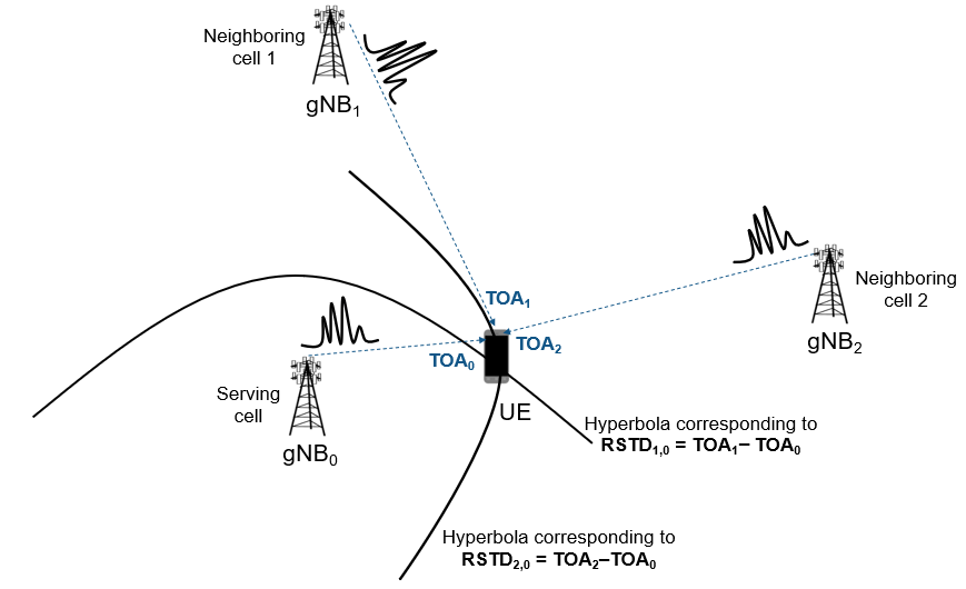
The OTDOA positioning approach is one of the downlink-based UE positioning techniques. This technique uses the reference signal timing difference (RSTD) or time difference of arrival (TDOA) measurements to perform multilateration or trilateration by using the theory of hyperbolas. The RSTD is the relative timing difference between the neighboring gNB and the reference gNB (which might be the serving cell), as defined in TS 38.215 Section 5.1.29 [1]. For the OTDOA technique, the PRS is transmitted by a set of neighboring gNBs along with the serving gNB. In this case, one gNB acts as a reference cell for the RSTD measurements. To avoid a synchronization error in RSTD measurements, all of the gNBs transmit the PRS at the same time (which means synchronized transmission from all gNBs). The time of arrival (TOA) of the PRS signals from different gNBs are estimated at the UE side. RSTD values are computed for a set of neighboring gNB and reference gNB pairs. An RSTD value between neighboring and reference is defined as, .
Each RSTD value that is obtained for a pair of gNBs corresponds to a hyperbola equation on which the UE is assumed to be located, with foci located at these gNBs. A set of hyperbola equations are deduced from a set of RSTD values, and the equations are solved to estimate the UE position. This process is called multilateration. The multilateration process involving one reference gNB and two neighboring gNBs is called trilateration (that is, the case of minimum requirement for UE positioning in 2-D).
This figure shows the positioning scenario with one reference gNB, which serves as the serving gNB, and two neighboring gNBs. The UE receives the PRS signals transmitted by all the gNBs at different timing instances (, , and ) based on the geographic distance and channel environment between the UE and gNBs. From this network of three gNBs, the system obtains two RSTD values from the TOA values. Each RSTD value corresponds to a hyperbola equation, on which the UE is assumed to be located. You can solve these two hyperbola equations to get UE position in 2-D.
This example shows how to create several gNB transmissions propagated through 38.901 channel and model the reception of the waveforms from all of the gNBs by one UE in urban macro ('UMa') path loss scenario. The UE performs correlation with the PRS to establish the delay from each gNB and subsequently the delay difference between the neighboring gNBs and reference gNB. These delay differences (RSTD values) are used to compute the hyperbolas of constant delay difference and are plotted relative to known gNB positions. The intersection of these hyperbolas is computed to estimate the position of the UE. This example focuses on the 2-D positioning estimate of a UE by assuming that all gNBs are synchronized. This example gives a better estimate for UE position when the UE is located near the center of gNBs network. This example assumes that all gNBs are operated at the same carrier frequency (which corresponds to a single positioning frequency layer). This example also assumes that all of the carriers have the same subcarrier spacing, cyclic prefix, and frequency allocation within the common resource grid.
Simulation Parameters
Specify the number of frames and the carrier frequency.
nFrames = 2; % Number of 10 ms frames
fc = 3e9;    % Carrier frequency (Hz)
Specify the number of gNBs in the range 3 to 19.
numgNBs = 7;
7;Carrier Configuration
Configure the carriers for all of the gNBs with different physical layer cell identities.
rng("default"); % Set RNG state for repeatability
cellIds = randperm(1008,numgNBs) - 1;

% Configure carrier properties
carrier = repmat(nrCarrierConfig,1,numgNBs);
for gNBIdx = 1:numgNBs
    carrier(gNBIdx).NCellID = cellIds(gNBIdx);
end
validateCarriers(carrier);
PRS Configuration
Configure PRS parameters for all of the gNBs. Configure the PRS for different gNBs such that no overlap exists to avoid the problem of hearability. For more information on how to configure PRS, see NR Positioning Reference Signal. This example considers different slot offsets for the PRS from different gNBs to avoid the overlap among PRS signals. This overlapping can be avoided in multiple ways by configuring the time-frequency aspects of PRS signals in an appropriate way (like choosing the nonoverlapped symbol allocation or frequency allocation, or by using muting pattern configuration parameters). This example transmits the PRS from each gNB in every alternate slot starting from slot 0 and considers the period as 2*numgNBs to accomodate the PRS resources from all the gNBs within one resource set period.
% Slot offsets of different PRS signals
prsSlotOffsets = 0:2:(2*numgNBs - 1);
prsIDs = randperm(4096,numgNBs) - 1;

% Configure PRS properties
prs = nrPRSConfig;
prs.PRSResourceSetPeriod = [2*numgNBs 0];
prs.PRSResourceOffset = 0;
prs.PRSResourceRepetition = 1;
prs.PRSResourceTimeGap = 1;
prs.MutingPattern1 = [];
prs.MutingPattern2 = [];
prs.NumRB = 52;
prs.RBOffset = 0;
prs.CombSize = 2;
prs.NumPRSSymbols = 12;
prs.SymbolStart = 0;
prs = repmat(prs,1,numgNBs);
for gNBIdx = 1:numgNBs
    prs(gNBIdx).PRSResourceOffset = prsSlotOffsets(gNBIdx);
    prs(gNBIdx).NPRSID = prsIDs(gNBIdx);
end
PDSCH Configuration
Configure the physical downlink shared channel (PDSCH) parameters for all of the gNBs for the data transmission. This example assumes that the data is transmitted from all of the gNBs that have a single transmission layer.
pdsch = nrPDSCHConfig;
pdsch.PRBSet = 0:51;
pdsch.SymbolAllocation = [0 14];
pdsch.DMRS.NumCDMGroupsWithoutData = 1;
pdsch = repmat(pdsch,1,numgNBs);
validateNumLayers(pdsch);
Channel and Thermal Noise Configuration
Specify the intersite distance in meters and use a seed to generate the gNB and UE positions within the site boundaries. This example creates a channel for urban macro (UMa) cellular scenario.
Scenario ="UMa"; % Deployment scenario ("UMi", "UMa", "RMa") interSiteDist = 500; % Intersite distance in meters SeedForPositions = 50; % Seed to generate the gNB and UE positions noiseFigure = 6; % Noise figure of the UE (dB) RxAntTemperature = 290; % Antenna temperature of the UE (K) applySmallScaleFading = true; % Flag to enable the small scale fading of the channel
To generate the scenario as mentioned in 3GPP TR 38.901, use h38901Scenario class.
s38901 = h38901Scenario(Scenario=Scenario,...
    IndoorRatio=[],...
    CarrierFrequency=fc,...             % Carrier frequency in Hz
    InterSiteDistance=interSiteDist,... % Intersite distance in meters
    NumCellSites=numgNBs,...            % Number of cell sites or gNBs
    NumSectors=1,...                    % Number of sectors per cell site
    NumUEs=1,...                        % Number of UEs
    Wrapping=false,...                  % Geographical distance-based wrapping
    Seed=SeedForPositions,...           % Seed to generate the gNB and UE positions
    LOSProbability=1);
Create all the channel links between each gNB and UE for the specified scenario.
% Get sample rate for the configured carrier(s). Assume sample rate is same
% for all carriers.
ofdmInfo = nrOFDMInfo(carrier(1));
[channels,channelInfo] = createChannelLinks(s38901,SampleRate=ofdmInfo.SampleRate,...
    FastFading=applySmallScaleFading);
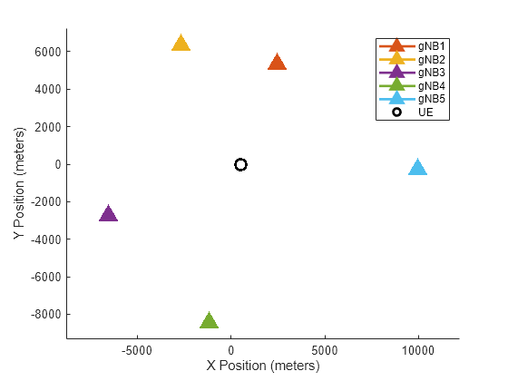
Visualize the UE and gNB positions.
gNBPos = channelInfo.AttachedUEInfo(1).Config.SitePositions;
UEPos = channelInfo.AttachedUEInfo(1).Config.UEPosition;
plotgNBAndUEPositions(gNBPos,UEPos,1:numgNBs,interSiteDist);
To allow the waveform to pass through the channel, enable channel filtering in all the channel links.
if applySmallScaleFading
    for gnbIdx = 1:numgNBs
        release(channels(gnbIdx).SmallScale);
        channels(gnbIdx).SmallScale.ChannelFiltering = true;
    end
end
This example configures the UE position in 3-D, but the position estimation algorithm computes the UE position in 2-D, considering the estimated height as 0 meters.
Generate PRS and PDSCH Resources
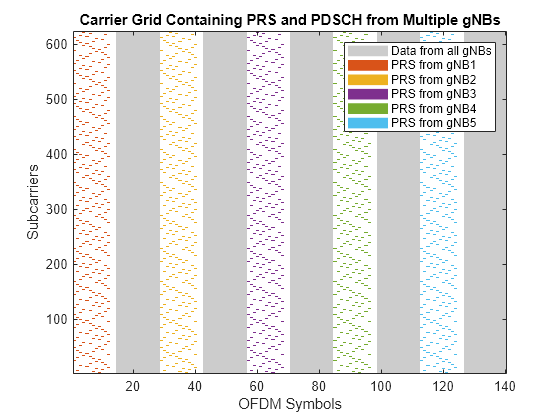
Generate PRS and PDSCH resources corresponding to all of the gNBs. To improve the hearability of PRS signals, transmit PDSCH resources in the slots in which the PRS is not transmitted by any of the gNBs. This example generates PRS and PDSCH resources with unit power (0 dB).
totSlots = nFrames*carrier(1).SlotsPerFrame;
prsGrid = cell(1,numgNBs);
dataGrid = cell(1,numgNBs);
for slotIdx = 0:totSlots-1
    [carrier(:).NSlot] = deal(slotIdx);
    [prsSym,prsInd] = deal(cell(1,numgNBs));
    for gNBIdx = 1:numgNBs
        % Create an empty resource grid spanning one slot in time domain
        slotGrid = nrResourceGrid(carrier(gNBIdx),1);

        % Generate PRS symbols and indices
        prsSym{gNBIdx} = nrPRS(carrier(gNBIdx),prs(gNBIdx));
        prsInd{gNBIdx} = nrPRSIndices(carrier(gNBIdx),prs(gNBIdx));

        % Map PRS resources to slot grid
        slotGrid(prsInd{gNBIdx}) = prsSym{gNBIdx};
        prsGrid{gNBIdx} = [prsGrid{gNBIdx} slotGrid];
    end
    % Transmit data in slots in which the PRS is not transmitted by any of
    % the gNBs (to control the hearability problem)
    for gNBIdx = 1:numgNBs
        dataSlotGrid = nrResourceGrid(carrier(gNBIdx),1);
        if all(cellfun(@isempty,prsInd))
            % Generate PDSCH indices
            [pdschInd,pdschInfo] = nrPDSCHIndices(carrier(gNBIdx),pdsch(gNBIdx));

            % Generate random data bits for transmission
            data = randi([0 1],pdschInfo.G,1);
            % Generate PDSCH symbols
            pdschSym = nrPDSCH(carrier(gNBIdx),pdsch(gNBIdx),data);

            % Generate demodulation reference signal (DM-RS) indices and symbols
            dmrsInd = nrPDSCHDMRSIndices(carrier(gNBIdx),pdsch(gNBIdx));
            dmrsSym = nrPDSCHDMRS(carrier(gNBIdx),pdsch(gNBIdx));

            % Map PDSCH and its associated DM-RS to slot grid
            dataSlotGrid(pdschInd) = pdschSym;
            dataSlotGrid(dmrsInd) = dmrsSym;
        end
        dataGrid{gNBIdx} = [dataGrid{gNBIdx} dataSlotGrid];
    end
end

% Plot carrier grid
plotGrid(prsGrid,dataGrid);
Generate Time-Domain Waveform
Perform orthogonal frequency-division multiplexing (OFDM) modulation of the signals at each gNB.
% Perform OFDM modulation of PRS and data signal at each gNB
txWaveform = cell(1,numgNBs);
for waveIdx = 1:numgNBs
    carrier(waveIdx).NSlot = 0;
    txWaveform{waveIdx} = nrOFDMModulate(carrier(waveIdx),prsGrid{waveIdx}+dataGrid{waveIdx});
end
Apply Channel
Calculate the propagation delay from each gNB to UE link in samples, using the known gNB and UE positions.
speedOfLight = physconst("LightSpeed"); % Speed of light in m/s
sampleDelay = zeros(1,numgNBs);
radius = zeros(1,numgNBs);
for gNBIdx = 1:numgNBs
   radius(gNBIdx) = rangeangle(gNBPos(gNBIdx,:)',UEPos');
   delay = radius(gNBIdx)/speedOfLight;               % Delay in seconds
   sampleDelay(gNBIdx) = delay*ofdmInfo.SampleRate;   % Delay in samples
end
Delay the waveform from each gNB and apply large-scale fading. If applySmallScaleFading is set to true, apply small-scale fading to the waveform. Then, at the UE, combine all the delayed and faded waveforms from all the gNBs
% Apply the propagation delays to all gNB transmissions
for gnbIdx = 1:numgNBs
    intSampleDelay = floor(sampleDelay(gnbIdx));
    staticDelay = dsp.Delay(Length=intSampleDelay);
    intSamplesDelayedTx = staticDelay(txWaveform{gnbIdx});

    variableFractionalDelay = dsp.VariableFractionalDelay(...
        InterpolationMethod="Farrow", ...
        FarrowSmallDelayAction="Use off-centered kernel", ...
        MaximumDelay=1);
    delayedWaveform{gnbIdx} = variableFractionalDelay(intSamplesDelayedTx,sampleDelay(gnbIdx)-intSampleDelay);
end
% Obtain the maximum possible channel delay
maxChDelay = 0;
if applySmallScaleFading
    % Obtain the maximum of maximum delays corresponding to all gNBs to UE links
    for gnbIdx = 1:numgNBs
        chInfo = info(channels(gnbIdx).SmallScale);
        maxChDelay = max(maxChDelay, chInfo.MaximumChannelDelay);
    end
end
rxWaveform = zeros(size(delayedWaveform{1},1)+maxChDelay,size(delayedWaveform{1},2));
for gnbIdx = 1:numgNBs
    % Pad the waveform to ensure the channel filter is fully flushed
    txWaveformPadded{gnbIdx} = [delayedWaveform{gnbIdx}; zeros(maxChDelay,1)];

    % Apply small-scale fading of the channel, if enabled
    if applySmallScaleFading
        [rxgNB{gnbIdx},pathGains] = channels(gnbIdx).SmallScale(txWaveformPadded{gnbIdx});
    else
        rxgNB{gnbIdx} = txWaveformPadded{gnbIdx}; %#ok<*UNRCH>
    end
    % Apply large-scale fading of the channel, i.e., Path loss
    rxgNB{gnbIdx} = rxgNB{gnbIdx}*db2mag(channels(gnbIdx).LargeScale);

    % Combine waveforms from all gNBs
    rxWaveform = rxWaveform + rxgNB{gnbIdx};
end
Add Noise
Generate and add the thermal noise to the received combined waveform at the UE end.
kBoltz = physconst("Boltzmann");             % Boltzmann constant
NF = db2pow(noiseFigure);                    % Noise figure in linear units
Teq = RxAntTemperature + 290*(NF-1);         % Equivalent noise temperature
N0 = sqrt(kBoltz*ofdmInfo.SampleRate*Teq/2); % Noise amplitude per receive antenna
% Generate thermal noise
noise = N0*complex(randn(size(rxWaveform)),randn(size(rxWaveform)));
% Add thermal noise to the received waveform
rxWaveform = rxWaveform + noise;
Estimate TOA
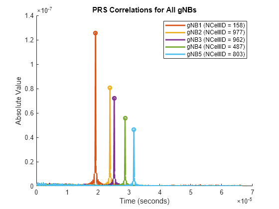
Configure the number of cells or gNBs to be detected for the multilateration process. This example does not consider the transmission of primary and secondary synchronization signals for the purpose of cell search. Instead, the UE performs the correlation on the incoming signal with reference PRS generated for each gNB, and cellsToBeDetected number of best cells are selected based on correlation outcome. Compute TOAs of the signals from each gNB by using nrTimingEstimate function. To estimate the position of UE, compute RSTD values by using the absolute TOAs corresponding to the best cells.
cellsToBeDetected = min(3,numgNBs);
if cellsToBeDetected < 3 || cellsToBeDetected > numgNBs
    error("nr5g:InvalidNumDetgNBs","The number of detected gNBs (" + num2str(cellsToBeDetected) + ...
        ") must be greater than or equal to 3 and less than or equal to the total number of gNBs (" + num2str(numgNBs) + ").");
end
corr = cell(1,numgNBs);
delayEst = zeros(1,numgNBs);
maxCorr = zeros(1,numgNBs);
for gNBIdx = 1:numgNBs
    [offset,mag] = nrTimingEstimate(carrier(gNBIdx),rxWaveform,prsGrid{gNBIdx});
    % Extract correlation data samples spanning about 1/14 ms for normal
    % cyclic prefix and about 1/12 ms for extended cyclic prefix (this
    % truncation is to ignore noisy side lobe peaks in correlation outcome)
    corr{gNBIdx} = mag(1:(ofdmInfo.Nfft*carrier(1).SubcarrierSpacing/15));
    % Delay estimate is at point of maximum correlation
    maxCorr(gNBIdx) = max(corr{gNBIdx});
    delayEst(gNBIdx) = find(corr{gNBIdx} == maxCorr(gNBIdx),1)-1;
end

% Get detected gNB numbers based on correlation outcome
[~,detectedgNBs] = sort(maxCorr,"descend");
detectedgNBs = detectedgNBs(1:cellsToBeDetected);

% Plot PRS correlation results
plotPRSCorr(carrier,corr,ofdmInfo.SampleRate);
Estimate UE Position Using OTDOA Technique
Calculate TDOA or RSTD values for all pairs of gNBs using the estimated TOA values by using the getRSTDValues function. Each RSTD value corresponding to a pair of gNBs can result from the UE being located at any position on a hyperbola with foci located at these gNBs.
% Compute RSTD values for multilateration or trilateration
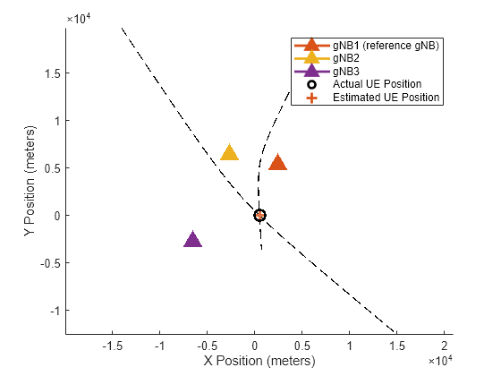
rstdVals = getRSTDValues(delayEst,ofdmInfo.SampleRate);Consider RSTD values corresponding to the detected gNBs for the estimation of the UE position. This example assumes the first detected gNB as the reference gNB and the others as neighboring gNBs. Calculate a set of hyperbola equations by using RSTD values corresponding to the pairs of reference gNB and neighboring gNBs. Plot the hyperbola equations, where the intersection of these curves represents the UE position. If you want to know which gNBs correspond to a hyperbola curve, you can know that information from the data tip in the figure.
% Plot gNB and UE positions
txCellIDs = [carrier(:).NCellID];
cellIdx = 1;
curveX = {};
curveY = {};
for jj = detectedgNBs(1) % Assuming first detected gNB as reference gNB
    for ii = detectedgNBs(2:end)
        rstd = rstdVals(ii,jj)*speedOfLight; % Delay distance
        % Establish gNBs for which delay distance is applicable by
        % examining detected cell identities
        txi = find(txCellIDs == carrier(ii).NCellID);
        txj = find(txCellIDs == carrier(jj).NCellID);
        if (~isempty(txi) && ~isempty(txj))
            % Get x- and y- coordinates of hyperbola curve and store them
            [x,y] = getRSTDCurve(gNBPos(txi,:,:),gNBPos(txj,:,:),rstd);
            if isreal(x) && isreal(y)
                curveX{1,cellIdx} = x; %#ok<*SAGROW>
                curveY{1,cellIdx} = y;

                % Get the gNB numbers corresponding to the current hyperbola
                % curve
                gNBNums{cellIdx} = [jj ii];
                cellIdx = cellIdx + 1;
            else
                warning("Due to the error in timing estimations, " + ...
                    "hyperbola curve cannot be deduced for the combination of gNB" + jj + " and gNB" + ii+". So, ignoring this gNB pair for the estimation of UE position.");
            end
        end
    end
end
numHyperbolaCurves = numel(curveX);
if numHyperbolaCurves < 2
    error('nr5g:InsufficientCurves',"The number of hyperbola curves ("+numHyperbolaCurves+") is not sufficient for the estimation of UE position in 2-D. Try with more number of gNBs.");
end
Use getEstimatedUEPosition function to estimate the UE position from the hyperbola curves. In general, two hyperbolas can intersect at, at most, two points. If there are two points of intersection, the algorithm in this example returns the average of two points of intersection for UE position estimation.
estimatedPos = getEstimatedUEPosition(curveX,curveY);

% Compute positioning estimation error
EstimationErr = norm(UEPos-estimatedPos); % in meters
disp("Estimated UE Position       : ["+ num2str(estimatedPos(1)) + " " + num2str(estimatedPos(2)) + "]" + newline + ...
      "UE Position Estimation Error: " + num2str(EstimationErr) + " meters");
Estimated UE Position       : [63.207 180.8384]
UE Position Estimation Error: 30.2567 meters
% Plot UE, gNB positions, and hyperbola curves
gNBsToPlot = unique([gNBNums{:}],"stable");
plotPositionsAndHyperbolaCurves(gNBPos,UEPos,gNBsToPlot,curveX,curveY,gNBNums,estimatedPos);
Summary and Further Exploration
This example shows OTDOA-based UE positioning estimation in 2-D.
You can vary the number of gNBs, locate the UE and gNBs at different positions.
You can also vary the time-frequency allocation parameters of PRS signals, vary the PDSCH configurations from each gNB, and see the variations in the estimated UE position.
References
3GPP TS 38.215. "NR; Physical layer measurements (Release 16)." 3rd Generation Partnership Project; Technical Specification Group Radio Access Network.
3GPP TR 38.901. “Study on channel model for frequencies from 0.5 to 100 GHz.” 3rd Generation Partnership Project; Technical Specification Group Radio Access Network.
Local Functions
This example uses these local functions to calculate gNB positions, validate carrier properties and the number of layers, estimate RSTD values, compute the UE position, and plot UE and gNB positions along with the generated hyperbolas.
function plotgNBAndUEPositions(gNBPos,UEPos,gNBNums,varargin)
%   plotgNBAndUEPositions(GNBPOS,UEPOS,GNBNUMS) plots gNB and UE positions.

    numgNBs = numel(gNBNums);
    colors = getColors(size(gNBPos,1));

    figure;
    hold on;
    legendstr = cell(1,numgNBs);

    % Plot position of each gNB
    for gNBIdx = 1:numgNBs
        plot3(gNBPos(gNBNums(gNBIdx),1),gNBPos(gNBNums(gNBIdx),2),gNBPos(gNBNums(gNBIdx),3), ...
            "Color",colors(gNBNums(gNBIdx),:),"Marker","^", ...
            "MarkerSize",11,"LineWidth",2,"MarkerFaceColor",colors(gNBNums(gNBIdx),:));
        legendstr{gNBIdx} = sprintf("gNB%d",gNBIdx);
    end

    % Plot UE position
    scatter3(UEPos(1),UEPos(2),UEPos(3),80,"LineWidth",2,"MarkerFaceColor","w","MarkerEdgeColor",[0 0.25 0.75],"MarkerFaceAlpha",0.2);view(2)

    if nargin == 4
        intersiteDistance = varargin{1};
        [sitex,sitey] = h38901Channel.sitePolygon(intersiteDistance);
        % Get bounding box of the union of the site polygons
        sysx = gNBPos(:,1) + sitex;
        sysy = gNBPos(:,2) + sitey;
        for gnbIdx = 1:numgNBs
            plot(sysx(gnbIdx,:),sysy(gnbIdx,:),"Color",[0 0.25 0.75],"LineStyle","-.");
            hold on;
        end

    end

    axis equal;
    legend([legendstr "UE"],"Location","bestoutside");
    xlabel("X Position (meters)");
    ylabel("Y Position (meters)");

end

function validateCarriers(carrier)
%   validateCarriers(CARRIER) validates the carrier properties of all
%   gNBs.

    % Validate physical layer cell identities
    cellIDs = [carrier(:).NCellID];
    if numel(cellIDs) ~= numel(unique(cellIDs))
        error("nr5g:invalidNCellID","Physical layer cell identities of all of the carriers must be unique.");
    end

    % Validate subcarrier spacings
    scsVals = [carrier(:).SubcarrierSpacing];
    if ~isscalar(unique(scsVals))
        error("nr5g:invalidSCS","Subcarrier spacing values of all of the carriers must be same.");
    end

    % Validate cyclic prefix lengths
    cpVals = {carrier(:).CyclicPrefix};
    if ~all(strcmpi(cpVals{1},cpVals))
        error("nr5g:invalidCP","Cyclic prefix lengths of all of the carriers must be same.");
    end

    % Validate NSizeGrid values
    nSizeGridVals = [carrier(:).NSizeGrid];
    if ~isscalar(unique(nSizeGridVals))
        error("nr5g:invalidNSizeGrid","NSizeGrid of all of the carriers must be same.");
    end

    % Validate NStartGrid values
    nStartGridVals = [carrier(:).NStartGrid];
    if ~isscalar(unique(nStartGridVals))
        error("nr5g:invalidNStartGrid","NStartGrid of all of the carriers must be same.");
    end

end

function validateNumLayers(pdsch)
%   validateNumLayers(PDSCH) validates the number of transmission layers,
%   given the array of physical downlink shared channel configuration
%   objects PDSCH.

numLayers = [pdsch(:).NumLayers];
if ~all(numLayers == 1)
    error("nr5g:invalidNLayers","The number of transmission layers"+ ...
        "configured for the data transmission must be 1.");
end
end

function plotPRSCorr(carrier,corr,sr)
%   plotPRSCorr(CARRIER,CORR,SR) plots PRS-based correlation for each gNB
%   CORR, given the array of carrier-specific configuration objects CARRIER
%   and the sampling rate SR.

    numgNBs = numel(corr);
    colors = getColors(numgNBs);
    figure;
    hold on;

    % Plot correlation for each gNodeB
    t = (0:length(corr{1}) - 1)/sr;
    legendstr = cell(1,2*numgNBs);
    for gNBIdx = 1:numgNBs
        plot(t,abs(corr{gNBIdx}), ...
            "Color",colors(gNBIdx,:),"LineWidth",2);
        legendstr{gNBIdx} = sprintf("gNB%d (NCellID = %d)", ...
            gNBIdx,carrier(gNBIdx).NCellID);
    end

    % Plot correlation peaks
    for gNBIdx = 1:numgNBs
        c = abs(corr{gNBIdx});
        j = find(c == max(c),1);
        plot(t(j),c(j),"Marker","o","MarkerSize",5, ...
            "Color",colors(gNBIdx,:),"LineWidth",2);
        legendstr{numgNBs+gNBIdx} = "";
    end
    legend(legendstr);
    xlabel("Time (seconds)");
    ylabel("Absolute Value");
    title("PRS Correlations for All gNBs");
end

function rstd = getRSTDValues(toa,sr)
%   RSTD = getRSTDValues(TOA,SR) computes RSTD values, given the time of
%   arrivals TOA and the sampling rate SR.

    % Compute number of samples delay between arrivals from different gNBs
    rstd = zeros(length(toa));
    for jj = 1:length(toa)
        for ii = 1:length(toa)
            rstd(ii,jj) = toa(ii) - toa(jj);
        end
    end

    % Get RSTD values in time
    rstd = rstd./sr;

end

function [x,y] = getRSTDCurve(gNB1,gNB2,rstd)
%   [X,Y] = getRSTDCurve(GNB1,GNB2,RSTD) returns the x- and y-coordinates
%   of a hyperbola equation corresponding to an RSTD value, given the pair
%   of gNB positions gNB1 and gNB2.

    % Calculate vector between two gNBs
    delta = gNB1 - gNB2;

    % Express distance vector in polar form
    [phi,r] = cart2pol(delta(1),delta(2));
    rd = (r+rstd)/2;

    % Compute the hyperbola parameters
    a = (r/2)-rd;         % Vertex
    c = r/2;              % Focus
    b = sqrt(c^2-a^2);    % Co-vertex
    hk = (gNB1 + gNB2)/2;
    mu = -2:1e-3:2;

    % Get x- and y- coordinates of hyperbola equation
    x = (a*cosh(mu)*cos(phi)-b*sinh(mu)*sin(phi)) + hk(1);
    y = (a*cosh(mu)*sin(phi)+b*sinh(mu)*cos(phi)) + hk(2);

end

function plotPositionsAndHyperbolaCurves(gNBPos,UEPos,detgNBNums,curveX,curveY,gNBNums,estPos)
%   plotPositionsAndHyperbolaCurves(GNBPOS,UEPOS,DETGNBNUMS,CURVEX,CURVEY,GNBNUMS,ESTPOS)
%   plots gNB, UE positions, and hyperbola curves by considering these
%   inputs:
%   GNBPOS     - Positions of gNBs
%   UEPOS      - Position of UE
%   DETGNBNUMS - Detected gNB numbers
%   CURVEX     - Cell array having the x-coordinates of hyperbola curves
%   CURVEY     - Cell array having the y-coordinates of hyperbola curves
%   GNBNUMS    - Cell array of gNB numbers corresponding to all hyperbolas
%   ESTPOS     - Estimated UE position

    plotgNBAndUEPositions(gNBPos,UEPos,detgNBNums);
    for curveIdx = 1:numel(curveX)
        curves(curveIdx) = plot(curveX{1,curveIdx},curveY{1,curveIdx}, ...
               "--","LineWidth",0.9,"Color",[0 0.25 0.75],"MarkerFaceColor","k");
    end
    % Add estimated UE position to figure
    plot3(estPos(1),estPos(2),estPos(3),"+","MarkerSize",10, ...
        "MarkerFaceColor","#D95319","MarkerEdgeColor","#D95319","LineWidth",2);

    % Add legend
    gNBLegends = cellstr(repmat("gNB",1,numel(detgNBNums)) + ...
        detgNBNums + [" (reference gNB)" repmat("",1,numel(detgNBNums)-1)]);
    legend([gNBLegends {'Actual UE Position'} repmat({''},1,numel(curveX)) {'Estimated UE Position'}]);

    for curveIdx = 1:numel(curves)
        % Create a data tip and add a row to the data tip to display
        % gNBs information for each hyperbola curve
        dt = datatip(curves(curveIdx));
        row = dataTipTextRow("Hyperbola of gNB" + gNBNums{curveIdx}(1) + ...
            " and gNB" + gNBNums{curveIdx}(2),'');
        curves(curveIdx).DataTipTemplate.DataTipRows = [row; curves(curveIdx).DataTipTemplate.DataTipRows];
        % Delete the data tip that is added above
        delete(dt);
    end

end

function colors = getColors(numgNBs)
%    COLORS = getColors(NUMGNBS) returns the RGB triplets COLORS for the
%    plotting purpose, given the number of gNBs NUMGNBS.

    % Form RGB triplets
    if numgNBs <= 10
        colors = [0.8500, 0.3250, 0.0980; 0.9290, 0.6940, 0.1250; 0.4940, 0.1840, 0.5560; ...
                  0.4660, 0.6740, 0.1880; 0.3010, 0.7450, 0.9330; 0.6350, 0.0780, 0.1840; ...
                  0.9290, 0.9, 0.3; 0.9290, 0.5, 0.9; 0.6660, 0.3740, 0.2880;0, 0.4470, 0.7410];
    else
        % Generate 30 more extra RGB triplets than required. It is to skip
        % the gray and white shades as these shades are reserved for the
        % data and no transmissions in carrier grid plot in this example.
        % With this, you can get unique colors for up to 1000 gNBs.
        colors = colorcube(numgNBs+30);
        colors = colors(1:numgNBs,:);
    end
end

function plotGrid(prsGrid,dataGrid)
%   plotGrid(PRSGRID,DATAGRID) plots the carrier grid from all gNBs.

    numgNBs = numel(prsGrid);
    figure()
    mymap = [1 1 1; ...       % White color for background
             0.8 0.8 0.8; ... % Gray color for PDSCH data from all gNBs
             getColors(numgNBs)];
    chpval = 3:numgNBs+2;

    gridWithPRS = zeros(size(prsGrid{1}));
    gridWithData = zeros(size(dataGrid{1}));
    names = cell(1,numgNBs);
    for gNBIdx = 1:numgNBs
        gridWithPRS = gridWithPRS + abs(prsGrid{gNBIdx})*chpval(gNBIdx);
        gridWithData = gridWithData + abs(dataGrid{gNBIdx});
        names{gNBIdx} = "PRS from gNB"+num2str(gNBIdx);
    end
    names = [{"Data from all gNBs"} names];
    % Replace all zero values of gridWithPRS with proper scaling (value of 1)
    % for white background
    gridWithPRS(gridWithPRS == 0) = 1;
    gridWithData(gridWithData ~=0) = 1;

    % Plot grid
    image(gridWithPRS+gridWithData); % In the resultant grid, 1 represents
                                     % the white background, 2 (constitute
                                     % of 1s from gridWithPRS and
                                     % gridWithData) represents PDSCH, and
                                     % so on
    % Apply colormap
    colormap(mymap);
    axis xy;

    % Generate lines
    L = line(ones(numgNBs+1),ones(numgNBs+1),"LineWidth",8);
    % Index colormap and associate selected colors with lines
    set(L,{"color"},mat2cell(mymap(2:numgNBs+2,:),ones(1,numgNBs+1),3)); % Set the colors

    % Create legend
    legend(names{:});

    % Add title
    title("Carrier Grid Containing PRS and PDSCH from Multiple gNBs");

    % Add labels to x-axis and y-axis
    xlabel("OFDM Symbols");
    ylabel("Subcarriers");
end

function estPos = getEstimatedUEPosition(xCell,yCell)
%   ESTPOS = getEstimatedUEPosition(XCELL,YCELL) returns the x-, y-, and z-
%   coordinates of the UE position, given the hyperbolas XCELL and YCELL.
%   Note that the z- coordinate is not estimated using this function but it
%   is returned as 0 meters.

    % Steps involved in this computation:
    % 1. Find closest points between hyperbolic surfaces
    % 2. Linearize surfaces around the points closest to intersection to
    % interpolate actual intersection location

    numCurves = numel(xCell);
    % Make all vectors have equal length
    maxLen = max(cellfun(@length,xCell));
    for curveIdx = 1:numCurves
        xCell{curveIdx} = [xCell{curveIdx} inf(1,maxLen-length(xCell{curveIdx}))];
        yCell{curveIdx} = [yCell{curveIdx} inf(1,maxLen-length(yCell{curveIdx}))];
    end
    tempIdx = 1;
    for idx1 = 1:numCurves-1
        for idx2 = (idx1+1):numCurves
            [firstCurve,secondCurve] = findMinDistanceElements(xCell{idx1},yCell{idx1},xCell{idx2},yCell{idx2});
            for idx3 = 1:numel(firstCurve)
                [x1a,y1a,x1b,y1b] = deal(firstCurve{idx3}(1,1),firstCurve{idx3}(1,2), ...
                                         firstCurve{idx3}(2,1),firstCurve{idx3}(2,2));
                [x2a,y2a,x2b,y2b] = deal(secondCurve{idx3}(1,1),secondCurve{idx3}(1,2), ...
                                         secondCurve{idx3}(2,1),secondCurve{idx3}(2,2));
                a1 = (y1b-y1a)/(x1b-x1a);
                b1 = y1a - a1*x1a;

                a2 = (y2b-y2a)/(x2b-x2a);
                b2 = y2a - a2*x2a;

                xC(tempIdx) = (b2-b1)/(a1-a2);
                yC(tempIdx) = a1*xC(tempIdx) + b1;
                tempIdx = tempIdx+1;
            end
        end
    end
    estPos = [mean(xC) mean(yC) 0];
end

function [firstCurvePoints,secondCurvePoints] = findMinDistanceElements(xA,yA,xB,yB)
%   [FIRSTCURVEPOINTS,SECONDCURVEPOINTS] = findMinDistanceElements(XA,YA,XB,YB)
%   returns the closest points between the given hyperbolic surfaces.

    distAB1 = zeros(numel(xA),numel(xB));
    for idx1 = 1:numel(xA)
        distAB1(idx1,:) = sqrt((xB-xA(idx1)).^2 + (yB-yA(idx1)).^2);
    end
    [~,rows] = min(distAB1,[],"omitnan");
    [~,col] = min(min(distAB1,[],"omitnan"));

    % Extract the indices of the points on two curves which are up to 5
    % meters apart. This is to identify the multiple intersections between
    % two hyperbola curves.
    [allRows,allCols] = find(distAB1 <= distAB1(rows(col),col)+5);
    diffVec = abs(allRows - allRows(1));
    index = find(diffVec > (min(diffVec) + max(diffVec))/2,1);
    allRows = [allRows(1);allRows(index)];
    allCols = [allCols(1);allCols(index)];

    for idx = 1:numel(allRows)
        firstCurveIndices = allRows(idx);
        secondCurveIndices = allCols(idx);
        x1a = xA(firstCurveIndices);
        y1a = yA(firstCurveIndices);
        x2a = xB(secondCurveIndices);
        y2a = yB(secondCurveIndices);

        % Use subsequent points to create line for linearization
        if firstCurveIndices == numel(rows)
            x1b = xA(firstCurveIndices-1);
            y1b = yA(firstCurveIndices-1);
        else
            x1b = xA(firstCurveIndices+1);
            y1b = yA(firstCurveIndices+1);
        end
        if secondCurveIndices == numel(rows)
            x2b = xB(secondCurveIndices-1);
            y2b = yB(secondCurveIndices-1);
        else
            x2b = xB(secondCurveIndices+1);
            y2b = yB(secondCurveIndices+1);
        end
        firstCurvePoints{idx} = [x1a y1a;x1b y1b]; %#ok<*AGROW>
        secondCurvePoints{idx} = [x2a y2a;x2b y2b];
    end
end