
Kernel Principal Component Analysis (KPCA)
MATLAB code for dimensionality reduction, fault detection, and fault diagnosis using KPCA.
이 제출물을 팔로우합니다
- 팔로우하는 게시물 피드에서 업데이트를 확인할 수 있습니다
- 정보 수신 기본 설정에 따라 이메일을 받을 수 있습니다
Kernel Principal Component Analysis (KPCA)
MATLAB code for dimensionality reduction, fault detection, and fault diagnosis using KPCA
Version 2.2, 14-MAY-2021
Email: iqiukp@outlook.com


Main features
- Easy-used API for training and testing KPCA model
- Support for dimensionality reduction, data reconstruction, fault detection, and fault diagnosis
- Multiple kinds of kernel functions (linear, gaussian, polynomial, sigmoid, laplacian)
- Visualization of training and test results
- Component number determination based on given explained level or given number
Notices
- Only fault diagnosis of Gaussian kernel is supported.
- This code is for reference only.
How to use
01. Kernel funcions
A class named Kernel is defined to compute kernel function matrix.
%{
        type   -

        linear      :  k(x,y) = x'*y
        polynomial  :  k(x,y) = (γ*x'*y+c)^d
        gaussian    :  k(x,y) = exp(-γ*||x-y||^2)
        sigmoid     :  k(x,y) = tanh(γ*x'*y+c)
        laplacian   :  k(x,y) = exp(-γ*||x-y||)


        degree -  d
        offset -  c
        gamma  -  γ
%}
kernel = Kernel('type', 'gaussian', 'gamma', value);
kernel = Kernel('type', 'polynomial', 'degree', value);
kernel = Kernel('type', 'linear');
kernel = Kernel('type', 'sigmoid', 'gamma', value);
kernel = Kernel('type', 'laplacian', 'gamma', value);
For example, compute the kernel matrix between X and Y
X = rand(5, 2);
Y = rand(3, 2);
kernel = Kernel('type', 'gaussian', 'gamma', 2);
kernelMatrix = kernel.computeMatrix(X, Y);
>> kernelMatrix

kernelMatrix =

    0.5684    0.5607    0.4007
    0.4651    0.8383    0.5091
    0.8392    0.7116    0.9834
    0.4731    0.8816    0.8052
    0.5034    0.9807    0.7274
02. Simple KPCA model for dimensionality reduction
clc
clear all
close all
addpath(genpath(pwd))
load('.\data\helix.mat', 'data')
kernel = Kernel('type', 'gaussian', 'gamma', 2);
parameter = struct('numComponents', 2, ...
'kernelFunc', kernel);
% build a KPCA object
kpca = KernelPCA(parameter);
% train KPCA model
kpca.train(data);
% mapping data
mappingData = kpca.score;
% Visualization
kplot = KernelPCAVisualization();
% visulize the mapping data
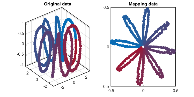
kplot.score(kpca)The training results (dimensionality reduction):
*** KPCA model training finished ***
running time            = 0.2798 seconds
kernel function         = gaussian
number of samples       = 1000
number of features      = 3
number of components    = 2
number of T2 alarm      = 135
number of SPE alarm     = 0
accuracy of T2          = 86.5000%
accuracy of SPE         = 100.0000%
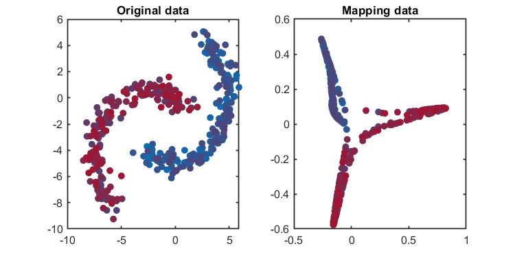
Another application using banana-shaped data:
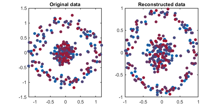
03. Simple KPCA model for reconstruction
clc
clear all
close all
addpath(genpath(pwd))

load('.\data\circle.mat', 'data')
kernel = Kernel('type', 'gaussian', 'gamma', 0.2);
parameter = struct('numComponents', 2, ...
                   'kernelFunc', kernel);
% build a KPCA object
kpca = KernelPCA(parameter);
% train KPCA model
kpca.train(data);

% reconstructed data
reconstructedData = kpca.newData;

% Visualization
kplot = KernelPCAVisualization();
kplot.reconstruction(kpca)
04. Component number determination
The Component number can be determined based on given explained level or given number.
Case 1
The number of components is determined by the given explained level. The given explained level should be 0 < explained level < 1. For example, when explained level is set to 0.75, the parameter should be set as:
parameter = struct('numComponents', 0.75, ...
                   'kernelFunc', kernel);
The code is
clc
clear all
close all
addpath(genpath(pwd))

load('.\data\TE.mat', 'trainData')
kernel = Kernel('type', 'gaussian', 'gamma', 1/128^2);

parameter = struct('numComponents', 0.75, ...
                   'kernelFunc', kernel);
% build a KPCA object
kpca = KernelPCA(parameter);
% train KPCA model
kpca.train(trainData);

% Visualization
kplot = KernelPCAVisualization();
kplot.cumContribution(kpca)
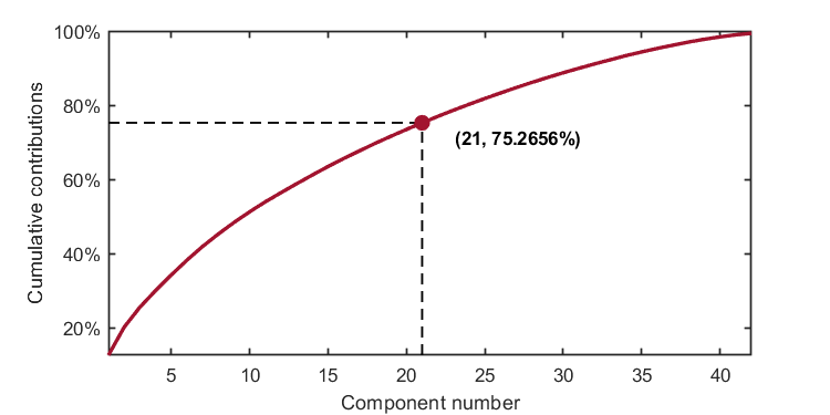
As shown in the image, when the number of components is 21, the cumulative contribution rate is 75.2656%,which exceeds the given explained level (0.75).
Case 2
The number of components is determined by the given number. For example, when the given number is set to 24, the parameter should be set as:
parameter = struct('numComponents', 24, ...
                   'kernelFunc', kernel);
The code is
clc
clear all
close all
addpath(genpath(pwd))

load('.\data\TE.mat', 'trainData')
kernel = Kernel('type', 'gaussian', 'gamma', 1/128^2);

parameter = struct('numComponents', 24, ...
                   'kernelFunc', kernel);
% build a KPCA object
kpca = KernelPCA(parameter);
% train KPCA model
kpca.train(trainData);

% Visualization
kplot = KernelPCAVisualization();
kplot.cumContribution(kpca)
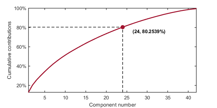
As shown in the image, when the number of components is 24, the cumulative contribution rate is 80.2539%.
05. Fault detection
Demonstration of fault detection using KPCA (TE process data)
clc
clear all
close all
addpath(genpath(pwd))
load('.\data\TE.mat', 'trainData', 'testData')
kernel = Kernel('type', 'gaussian', 'gamma', 1/128^2);
parameter = struct('numComponents', 0.65, ...
'kernelFunc', kernel);
% build a KPCA object
kpca = KernelPCA(parameter);
% train KPCA model
kpca.train(trainData);
% test KPCA model
results = kpca.test(testData);
% Visualization
kplot = KernelPCAVisualization();
kplot.cumContribution(kpca)
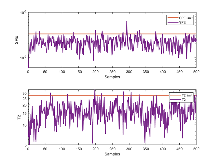
kplot.trainResults(kpca)
kplot.testResults(kpca, results)The training results are
*** KPCA model training finished ***
running time            = 0.0986 seconds
kernel function         = gaussian
number of samples       = 500
number of features      = 52
number of components    = 16
number of T2 alarm      = 16
number of SPE alarm     = 17
accuracy of T2          = 96.8000%
accuracy of SPE         = 96.6000%
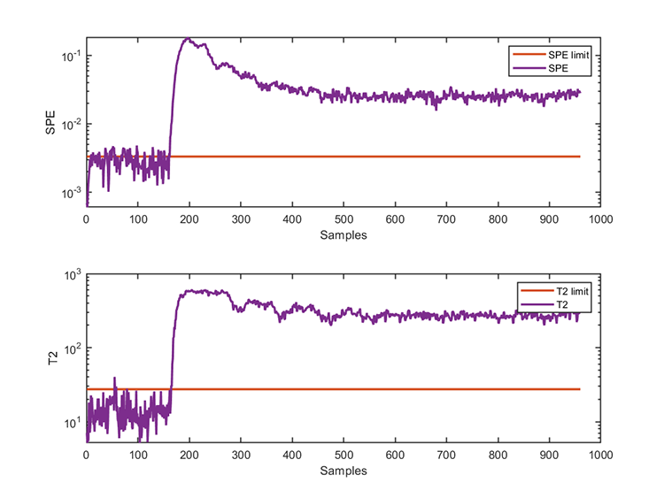
The test results are
*** KPCA model test finished ***
running time            = 0.0312 seconds
number of test data     = 960
number of T2 alarm      = 799
number of SPE alarm     = 851
06. Fault diagnosis
Notice
- If you want to calculate CPS of a certain time, you should set starting time equal to ending time. For example, 'diagnosis', [500, 500]
- If you want to calculate the average CPS of a period of time, starting time and ending time should be set respectively. 'diagnosis', [300, 500]
- The fault diagnosis module is only supported for gaussian kernel function and it may still take a long time when the number of the training data is large.
clc
clear all
close all
addpath(genpath(pwd))
load('.\data\TE.mat', 'trainData', 'testData')
kernel = Kernel('type', 'gaussian', 'gamma', 1/128^2);
parameter = struct('numComponents', 0.65, ...
'kernelFunc', kernel,...
'diagnosis', [300, 500]);
% build a KPCA object
kpca = KernelPCA(parameter);
% train KPCA model
kpca.train(trainData);
% test KPCA model
results = kpca.test(testData);
% Visualization
kplot = KernelPCAVisualization();
kplot.cumContribution(kpca)
kplot.trainResults(kpca)
kplot.testResults(kpca, results)
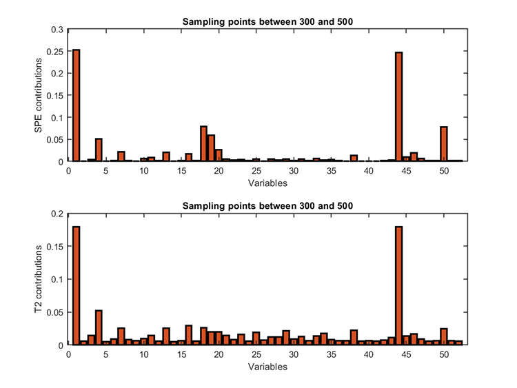
kplot.diagnosis(results)Diagnosis results:
*** Fault diagnosis ***
Fault diagnosis start...
Fault diagnosis finished.
running time            = 18.2738 seconds
start point             = 300
ending point            = 500
fault variables (T2)    = 44   1   4
fault variables (SPE)   = 1  44  18
인용 양식
Kepeng Qiu (2026). Kernel Principal Component Analysis (KPCA) (https://github.com/iqiukp/KPCA-MATLAB), GitHub. 검색 날짜: .
일반 정보
- 버전 2.2.1 (988 KB)
-
 GitHub에서 라이선스 보기
MATLAB 릴리스 호환 정보
- R2016b 이상 릴리스와 호환
플랫폼 호환성
- Windows
- macOS
- Linux
GitHub 디폴트 브랜치를 사용하는 버전은 다운로드할 수 없음
| 버전 | 퍼블리시됨 | 릴리스 정보 | Action |
|---|---|---|---|
| 2.2.1 | * Added descriptions |
||
| 2.2 | Please visit https://github.com/iqiukp/Kernel-Principal-Component-Analysis-KPCA for detailed information. |
||
| 2.1.2 | 1. Added some descriptions |
||
| 2.1.1 | 1. Added some descriptions |
||
| 2.1 | 1. added support for data reconstruction |
||
| 2.0 | 1. Used OOP to rewrite some modules.
|
||
| 1.2 | 1. Fixed some errors
|
||
| 1.1.1 | 1. Fixed some errors
|
||
| 1.1 | 1. Fixed some errors
|
||
| 1.0.0 |