AODV Routing in TDMA-Based MANET
This example shows how to simulate a multihop wireless scenario in a time division multiple access (TDMA) based mobile ad hoc network (MANET) by using the ad hoc on-demand distance vector (AODV) routing protocol and evaluate the network performance.
Using this example, you can:
Create and configure TDMA nodes to set up a MANET scenario.
Add application traffic to nodes.
Configure the AODV routing protocol and add it to TDMA nodes.
Simulate the MANET scenario and visualize the node topology.
Capture and visualize application layer (APP), medium access control (MAC) layer, and physical layer (PHY) statistics for each node.
Visualize the routes established by the AODV routing protocol.
Additionally, this example script enables you to add fixed routing paths and display the routing table of a node. For more information, see Further Exploration.
AODV Routing Protocol
The AODV routing protocol operates as a dynamic, self-starting protocol designed for MANETs. It is a reactive routing protocol that establishes routes only when the data packet transmission from a source to a destination is necessary. AODV uses route discovery and route maintenance processes to efficiently adapt to network topology changes. During route discovery, nodes establish a communication path between the source and destination by transmitting the route request (RREQ) and route reply (RREP) messages. To inform nodes of link failures and implement local route repair mechanisms, AODV uses route error (RERR) messages. Further, AODV sends periodic HELLO messages to maintain local connectivity and detect link breakages, thereby ensuring robust communication in dynamic environments. For more information, see RFC 3561 [1].
Simulation Scenario
The example simulates this MANET scenario consisting of 10 TDMA nodes.
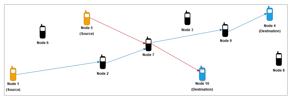
Node 1 and Node 5 act as source nodes, while Node 4 and Node 10 are their respective destination nodes. Initially, the AODV routing protocol establishes routes from Node 1 to Node 4 through Node 2, Node 7, and Node 9 and from Node 5 to Node 10 via Node 7.
This figure shows how node mobility continuously changes the topology of the MANET scenario.
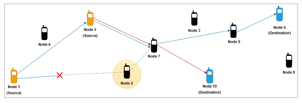
Due to the mobility of Node 2, the link between Node 1 and Node 2 breaks. In response, AODV dynamically reconfigures the route from the source Node 1 to destination Node 4, redirecting traffic through Node 5, Node 7, and Node 9.
Create and Configure Scenario
Set the seed for the random number generator to 1 to ensure repeatability. The seed value controls the pattern of random number generation. The random number generated by the seed value impacts several processes within the simulation, including predicting packet reception success at the physical layer. To improve the accuracy of your simulation results after running the simulation, you can change the seed value, run the simulation again, and average the results over multiple simulations.
rng(1,"combRecursive")Specify the simulation time in seconds. Initialize the wireless network simulator.
simulationTime = 50;
networkSimulator = wirelessNetworkSimulator.init;
50;
networkSimulator = wirelessNetworkSimulator.init;Nodes and Transmission Slots
Create and configure 10 TDMA nodes, specifying their positions (in meters) and names. Specify the transmission power (in dBm) and number of slots per frame for all the TDMA nodes.
nodePositions = [10 350 0; 800 400 0; 1600 750 0; ...
    2300 800 0; 570 750 0; 250 650 0; 1200 500 0; ...
    2400 400 0; 1900 580 0; 1750 230 0];
nodeNames = ["Node1","Node2","Node3","Node4","Node5", ...
    "Node6","Node7","Node8","Node9","Node10"];
nodes = hTDMANode(Position=nodePositions,Name=nodeNames,TransmitPower=10);
tdmaConfig = hTDMAConfig(NumSlotsPerFrame=size(nodePositions,1));
configureTDMA(nodes,tdmaConfig)
Assign transmission slots to nodes.
assignSlot(nodes)
AODV Routing
By default, TDMA nodes use a default AODV configuration as their routing protocol. Set the NETDiameter property in AODV to specify the maximum number of hops a packet can traverse in the network. The default value is 35. You can also configure these AODV properties.
AllowedHelloLoss— Specifies the maximum number of consecutive hello messages a node can lose before it marks the route as broken. The default value is2.HelloInterval— Specifies the periodicity of Hello messages. Units are in seconds. The default value is1.ActiveRouteTimeout— Specifies how long a node keeps the route active after its last use. Units are in seconds. The default value is3.MaxRouteRequestRetries— Specifies the maximum number of retries allowed for route request packets. The default value is2.EnableLocalRepair— Enables the local repair mechanism when a route breaks. The local repair mechanism enables an intermediate node to repair a broken route to the destination node without notifying the source node. The default value istrue.
aodv = hAODVRouting(NETDiameter=8);
addMeshRouting(nodes,aodv)
Application Traffic
Generate an On-Off application traffic pattern by using the networkTrafficOnOff object. Configure the On-Off application traffic by specifying the application data rate (in kbps), on time (in seconds), and off time (in seconds). Add application traffic from Node 1 to Node 4 and from Node 5 to Node 10.
srcNodes = [nodes(1) nodes(5)];
dstNodes = [nodes(4) nodes(10)];
traffic = networkTrafficOnOff(DataRate=800,OnTime=0.7,OffTime=0.3);
addTrafficSource(srcNodes(1),traffic,DestinationNode=dstNodes(1))

traffic = networkTrafficOnOff(DataRate=400,OnTime=0.7,OffTime=0.3);
addTrafficSource(srcNodes(2),traffic,DestinationNode=dstNodes(2))
Mobility
Add random waypoint mobility to all nodes except Node 2.
addMobility([nodes(1) nodes(3:10)],MobilityModel="random-waypoint",RefreshInterval=0.1)To move Node 2 out of the network during the simulation, add constant velocity mobility model to it.
addMobility(nodes(2),MobilityModel="constant-velocity",Velocity=[5 0 0],RefreshInterval=0.1)Visualization
To view the live network topology, set enableNetworkVisualization to true. To visualize state transition at the nodes as they transmit and receive packets, set enablePacketVisualization to true. To visualize the live queued packet count in the transmit buffer of nodes, set enableMetricVisualization to true.
enableNetworkVisualization =true; enablePacketVisualization =
false; enableMetricVisualization =
true;
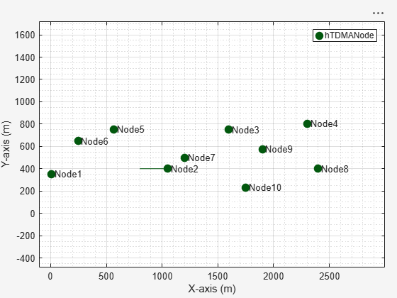
Visualize the network topology by using the wirelessNetworkViewer object.
if enableNetworkVisualization
visualizerObj = wirelessNetworkViewer;
addNodes(visualizerObj,nodes)
end
Visualize the state transition at the nodes by using the wirelessTrafficViewer object. To view the state transition at the nodes at the end of the simulation, set the RefreshRate property to 0. To visualize live state transitions during the simulation, set the RefreshRate property to a positive integer. Note that enabling live state transition with higher refresh rate proportionally increases the simulation runtime.
if enablePacketVisualization
    packetVisObj = wirelessTrafficViewer(ViewType="state-transition-plot",RefreshRate=0);
    addNodes(packetVisObj,nodes)
    hRegisterTDMAToTrafficViewer(packetVisObj,nodes)
end
Visualize the queued packet count in the transmit buffer of nodes by using the helperMetricsVisualizer helper function.
if enableMetricVisualization
    metricsVisObj = helperMetricsVisualizer(nodes,RefreshRate=2);
end
Simulation and Results
Add nodes to the wireless network simulator.
addNodes(networkSimulator,nodes)
To calculate the application throughput, application packet delivery ratio (PDR), routing overhead, and average end-to-end delay of the network, use the helperTDMAKPIManager helper object.
performanceObj = helperTDMAKPIManager(nodes,["app-throughput","app-packet-delivery-ratio","app-average-end-to-end-delay","routing-overhead"],LogInterval=1);
Display the routes that the AODV routing protocol establishes for each source-destination pair by scheduling a periodic action at every 5 seconds in the wireless network simulator.
scheduleAction(networkSimulator,@(actionID,srcDstPair) helperDisplayRoutes(srcDstPair),[srcNodes(1) dstNodes(1);srcNodes(2) dstNodes(2)],0,5);
Run the simulation for the specified simulation time.
run(networkSimulator,simulationTime)
At t = 0.000000 seconds
No route exists from Node1 to Node4
No route exists from Node5 to Node10
............................................................
At t = 5.000000 seconds
Node1 -> Node2 -> Node7 -> Node9 -> Node4
Node5 -> Node7 -> Node10
............................................................
At t = 10.000000 seconds
Node1 -> Node2 -> Node7 -> Node9 -> Node4
Node5 -> Node7 -> Node10
............................................................
At t = 15.000000 seconds
Node1 -> Node2 -> Node7 -> Node9 -> Node4
Node5 -> Node7 -> Node10
............................................................
At t = 20.000000 seconds
Node1 -> Node2 -> Node7 -> Node9 -> Node4
Node5 -> Node7 -> Node10
............................................................
At t = 25.000000 seconds
Node1 -> Node2 -> Node7 -> Node9 -> Node4
Node5 -> Node7 -> Node10
............................................................
At t = 30.000000 seconds
Node1 -> Node2 -> Node7 -> Node9 -> Node4
Node5 -> Node7 -> Node10
............................................................
At t = 35.000000 seconds
Node1 -> Node5 -> Node7 -> Node9 -> Node4
Node5 -> Node7 -> Node10
............................................................
At t = 40.000000 seconds
Node1 -> Node5 -> Node7 -> Node9 -> Node4
Node5 -> Node7 -> Node10
............................................................
At t = 45.000000 seconds
Node1 -> Node5 -> Node7 -> Node9 -> Node4
Node5 -> Node7 -> Node10
............................................................
At t = 50.000000 seconds
Node1 -> Node5 -> Node7 -> Node9 -> Node4
Node5 -> Node7 -> Node10
............................................................
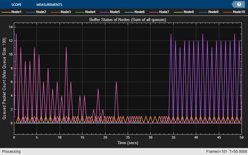
The metric visualizer shows:
Node 7 accumulates a higher packet count in its transmit queue between 0 and 23 seconds because it functions as a relay node on the paths from Node 1 to Node 4 and from Node 5 to Node 10. Node 7 buffers all packets originating from Node 1 and Node 5 for forwarding to their respective destination nodes.
Between 23 and 34 seconds, the packet count in the transmit queue of Node 7 decreases as the route from Node 1 to Node 4 becomes unavailable because Node 2 exits the network. After 34 seconds, the network reestablishes the route through Node 5. Consequently, the transmit queue of Node 5 experiences a higher packet count because Node 5 acts as both a relay on the path from Node 1 to Node 4 and a source node.
Retrieve the APP, MAC, and PHY statistics at each node.
stats = statistics(nodes);
Calculate the throughput, PDR, routing overhead, and average end-to-end delay of the network.
Network throughput measures the rate at which the source nodes successfully deliver application data bytes to their destination nodes. Units are in Mbps.
networkThroughput = kpi(performanceObj,[],[],"app-throughput")networkThroughput = 0.7254
Packet delivery ratio is the ratio of application data packets successfully delivered at the destination nodes to the total number of application data packets transmitted by the source nodes.
pdr = kpi(performanceObj,[],[],"app-packet-delivery-ratio")pdr = 0.8633
Routing overhead is the ratio of total number of routing packets to the total number of packets transmitted in the network.
routingOverheadVal = kpi(performanceObj,[],[],"routing-overhead")routingOverheadVal = 0.0404
Average end-to-end delay is the average time it takes for a data packet to travel from the source node to the destination node, in seconds.
avgEndToEndDelay = kpi(performanceObj,[],[],"app-average-end-to-end-delay")avgEndToEndDelay = 0.0676
Plot and visualize these APP, MAC, and PHY statistics at each node.
Transmitted and received packets at the APP.
Transmitted, received, and unintended received packets at the MAC layer. If the node is not the intended receiver, the MAC layer discards any packet it receives from the PHY.
Transmitted, received, and decode-failed packets at the PHY.
helperStatisticsVisualizer(nodes);
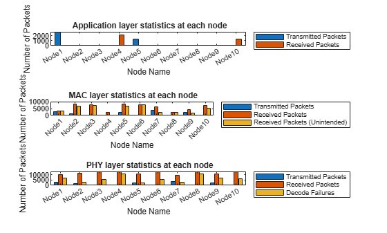
At the APP, Node 1 and Node 5 transmit packets, while Node 4 and Node 10 receive packets.
At the MAC layer, the source nodes and the nodes located along the paths to the destination nodes, transmit packets.
Visualize the variation of instantaneous application throughput (in Mbps) from Node 1 to Node 4 in every one-second interval.
figure('Name',"Instantaneous Application Throughput");
instantaneousAppThroughput = zeros(1,simulationTime);
sampleTimes = 1:simulationTime;
for currTime = sampleTimes
    instantaneousAppThroughput(currTime) = kpi(performanceObj,nodes(1),nodes(4),"app-throughput",StartTime=currTime-1,EndTime=currTime);
end
plot(sampleTimes, instantaneousAppThroughput, '-', 'LineWidth', 1.5);
xlabel('Time (s)');
ylabel('Instantaneous APP Throughput (Mbps)');
title('Instantaneous Application Throughput');
legend('App-Throughput from Node 1 to Node 4');
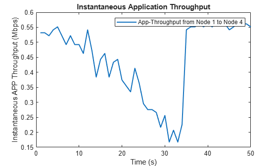
The plot shows that the instantaneous application throughput from Node 1 to Node 4. The throughput drops between 23 and 34 seconds because Node 2 exits the network. After 34 seconds, the throughput recovers because the network reestablishes the route from Node 1 to Node 4 via Node 5.
In summary, the simulation results presented in this example show that packets traverse the routes established by the AODV routing protocol, moving from the source node to the destination node via the intermediate relay nodes.
Further Exploration
You can use this example to further explore these functionalities.
Add Fixed Routing Paths
To establish a fixed mesh path from the source node to the destination node through the intermediate nodes, use the addFixedMeshPath function of the hTDMANode helper object. When selecting a route for packet transmission to the destination, the source node prioritizes the fixed mesh routing paths over those established by the mesh routing protocol. However, both types of routes coexist within the network.
To add a path from Node 1 to Node 4 through Node 2 and Node 3, uncomment this code and add it after you create the nodes.
% nextHopNodes = nodes(2:3);
% addFixedMeshPath(nodes(1),nodes(4),nextHopNodes)
Display Routing Table
To display the routes that AODV establishes and the addFixedMeshPath function adds to a node, use the meshRoutingTable function of the hTDMANode helper object. Uncomment this code and add it after you start running the simulation.
% [fixedMeshRouteTable,dynamicRoutingTable] = meshRoutingTable(nodes(1))Supporting Functions
The example uses these helper functions and objects:
hTDMANode— Creates a TDMA nodehTDMAConfig— Creates a TDMA frame configuration objecthTDMANodeMesh— Implements mesh layer functionalityhTDMANodeMAC— Implements TDMA-based MAC functionalityhTDMANodePHY— Implements TDMA-based PHY functionalityhIntraNodeScheduler— Performs the scheduled operations of the nodehelperPacketDuplicateDetector— Detects duplicate packetshAODVRouting— Implements the AODV routing protocolhTDMANodeEventCallback— Invokes registered callbacks for the eventshelperTDMAKPIManager— Computes key performance indicators (KPI) of the TDMA networkhelperDisplayRoutes— Displays routes established for a given source-destination pairhelperMetricsVisualizer— Plots MAC layer metricshelperStatisticsVisualizer— Plots the APP, MAC, and PHY statistics of each node
References
Das, Samir R., Charles E. Perkins, and Elizabeth M. Belding-Royer. Ad Hoc On-Demand Distance Vector (AODV) Routing. Request for Comments RFC 3561. Internet Engineering Task Force, 2003. https://datatracker.ietf.org/doc/rfc3561/.
See Also
Objects
wirelessNetworkSimulator|wirelessTrafficViewer|wirelessNetworkViewer|networkTrafficOnOff|nodeMobilityRandomWalk|nodeMobilityRandomWaypoint|nodeMobilityConstantVelocity