Wavelet Cross-Correlation for Lead-Lag Analysis
This example shows how to use wavelet cross-correlation to measure similarity between two signals at different scales.
Wavelet cross-correlation is simply a scale-localized version of the usual cross-correlation between two signals. In cross-correlation, you determine the similarity between two sequences by shifting one relative to the other, multiplying the shifted sequences element by element and summing the result. For deterministic sequences, you can write this as an ordinary inner product: where and are sequences (signals) and the bar denotes complex conjugation. The variable, k, is the lag variable and represents the shift applied to . If both and are real, the complex conjugate is not necessary. Assume that is the same sequence as but delayed by L>0 samples, where L is an integer. For concreteness, assume . If you express in terms of above, you obtain . By the Cauchy-Schwartz inequality, the above is maximized when . This means if you left shift (advance) by 10 samples, you get the maximum cross-correlation sequence value. If is a L-delayed version of , , then the cross-correlation sequence is maximized at . You can show this by using xcorr.
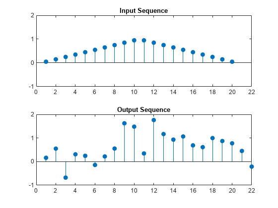
Create a triangular signal consisting of 20 samples. Create a noisy shifted version of this signal. The shift in the peak of the triangle is 3 samples. Plot the x and y sequences.
n = 20;
x0 = 1:n/2;
x1 = (2*x0-1)/n;
x = [x1 fliplr(x1)]';
rng default;
y = [zeros(3,1);x]+0.3*randn(length(x)+3,1);

subplot(2,1,1)
stem(x,'filled')
axis([0 22 -1 2])
title('Input Sequence')

subplot(2,1,2)
stem(y,'filled')
axis([0 22 -1 2])
title('Output Sequence')
Use xcorr to obtain the cross-correlation sequence and determine the lag where the maximum is obtained.
[xc,lags] = xcorr(x,y);
[~,I] = max(abs(xc));
figure
stem(lags,xc,'filled')
legend(sprintf('Maximum at lag %d',lags(I)))
title('Sample Cross-Correlation Sequence')
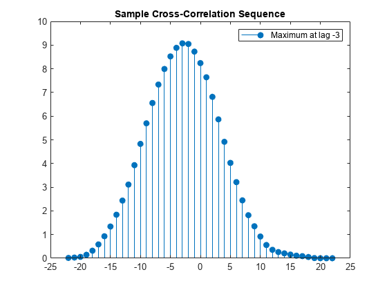
The maximum is found at a lag of -3. The signal y is the second input to xcorr and it is a delayed version of x. You have to shift y 3 samples to the left (a negative shift) to maximize the cross correlation. If you reverse the roles of x and y as inputs to xcorr, the maximum lag now occurs at a positive lag.
[xc,lags] = xcorr(y,x);
[~,I] = max(abs(xc));
figure
stem(lags,xc,'filled')
legend(sprintf('Maximum at lag %d',lags(I)))
title('Sample Cross-Correlation Sequence')
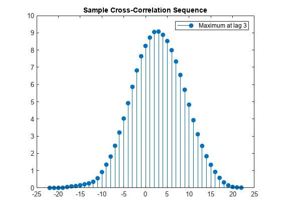
x is an advanced version of y and you delay x by three samples to maximize the cross correlation.
modwtxcorr is the scale-based version of xcorr. To use modwtxcorr, you first obtain the nondecimated wavelet transforms.
Apply wavelet cross-correlation to two signals that are shifted versions of each other. Construct two exponentially-damped 200-Hz sine waves with additive noise. The x signal has its time center at seconds while y is centered at seconds.
t = 0:1/2000:1-1/2000;
x = sin(2*pi*200*t).*exp(-50*pi*(t-0.2).^2)+0.1*randn(size(t));
y = sin(2*pi*200*t).*exp(-50*pi*(t-0.5).^2)+0.1*randn(size(t));
figure
plot(t,x)
hold on
plot(t,y)
xlabel('Seconds')
ylabel('Amplitude')
grid on
legend('x','y')
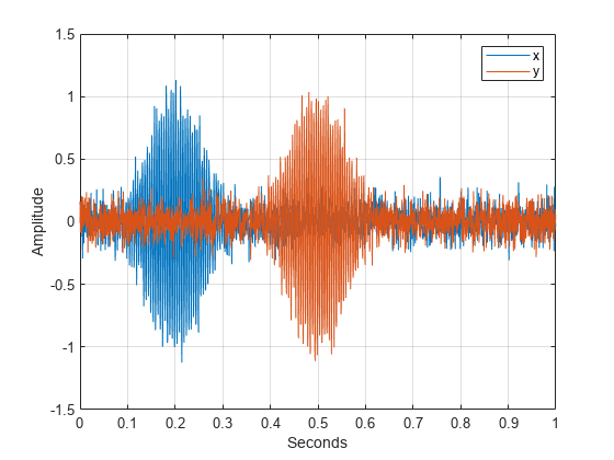
You see that x and y are very similar except that y is delayed by 0.3 seconds. Obtain the nondecimated wavelet transform of x and y down to level 5 using the Fejér-Korovkin (14) wavelet. The wavelet coefficients at level 3 with a sampling frequency of 2 kHz are an approximate bandpass filtering of the inputs. The frequency localization of the Fejér-Korovkin filters ensures that this bandpass approximation is quite good.
wx = modwt(x,'fk14',5);
wy = modwt(y,'fk14',5);
Obtain the wavelet cross-correlation sequences for the wavelet transforms of x and y. Plot the level 3 wavelet cross-correlation sequence for 2000 lags centered at zero lag. Multiply the lags by the sampling period to obtain a meaningful time axis.
[xc,~,lags] = modwtxcorr(wx,wy,'fk14');
lev = 3;
zerolag = floor(numel(xc{lev})/2+1);
tlag = lags{lev}(zerolag-999:zerolag+1000).*(1/2000);
figure
plot(tlag,xc{lev}(zerolag-999:zerolag+1000))
title('Wavelet Cross-Correlation Sequence (level 3)')
xlabel('Time')
ylabel('Cross-Correlation Coefficient')
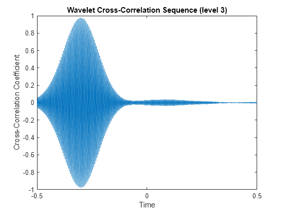
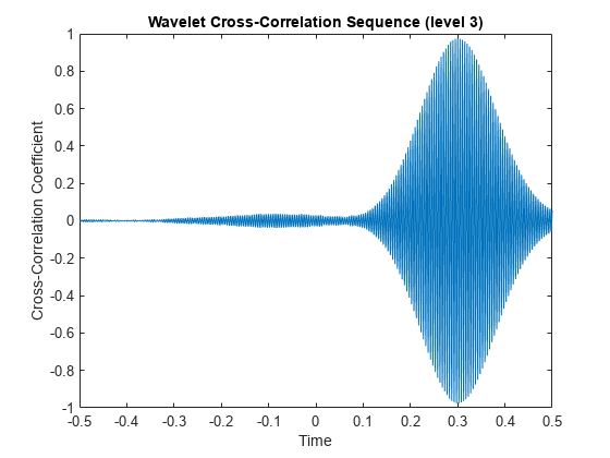
The cross-correlation sequence peaks at a delay of -0.3 seconds. The wavelet transform of y is the second input to modwtxcorr. Because the second input of modwtxcorr is shifted relative to the first, the peak correlation occurs at a negative delay. You have to left shift (advance) the cross-correlation sequence to align the time series. If you reverse the roles of the inputs to modwtxcorr, you obtain the peak correlation at a positive lag.
[xc,~,lags] = modwtxcorr(wy,wx,'fk14');
lev = 3;
zerolag = floor(numel(xc{lev})/2+1);
tlag = lags{lev}(zerolag-999:zerolag+1000).*(1/2000);
figure
plot(tlag,xc{lev}(zerolag-999:zerolag+1000))
title('Wavelet Cross-Correlation Sequence (level 3)')
xlabel('Time')
ylabel('Cross-Correlation Coefficient')
To show that wavelet cross-correlation enables scale(frequency)-localized correlation, plot the cross-correlation sequences at levels 1 and 5.
lev = 1;
zerolag = floor(numel(xc{lev})/2+1);
tlag = lags{lev}(zerolag-999:zerolag+1000).*(1/2000);
plot(tlag,xc{lev}(zerolag-999:zerolag+1000))
title('Wavelet Cross-Correlation Sequence (level 1)')
xlabel('Time')
ylabel('Cross-Correlation Coefficient')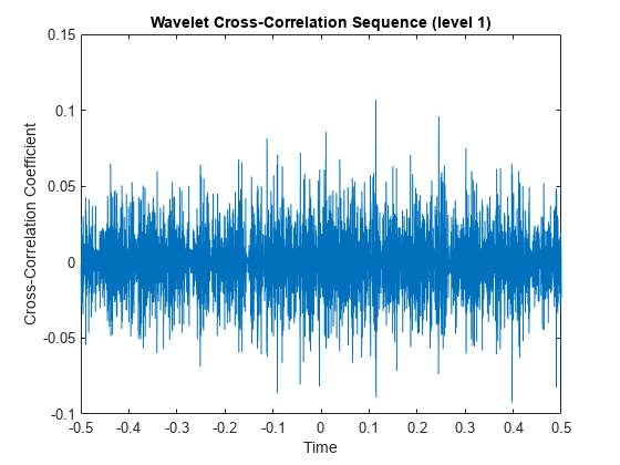
figure
lev = 5;
zerolag = floor(numel(xc{lev})/2+1);
tlag = lags{lev}(zerolag-999:zerolag+1000).*(1/2000);
plot(tlag,xc{lev}(zerolag-999:zerolag+1000))
title('Wavelet Cross-Correlation Sequence (level 5)')
xlabel('Time')
ylabel('Cross-Correlation Coefficient')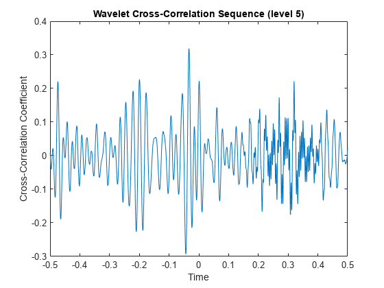
The wavelet cross-correlation sequences at levels 1 and 5 do not show any evidence of the exponentially-weighted sinusoids due to the bandpass nature of the wavelet transform.
With financial data, there is often a leading or lagging relationship between variables. In those cases, it is useful to examine the cross-correlation sequence to determine if lagging one variable with respect to another maximizes their cross-correlation. To illustrate this, consider the correlation between two components of the GDP -- personal consumption expenditures and gross private domestic investment. The data is quarterly chain-weighted U.S. real GDP data for 1974Q1 to 2012Q4. The data were transformed by first taking the natural logarithm and then calculating the year-over-year difference. Look at the correlation between two components of the GDP -- personal consumption expenditures, pc, and gross private domestic investment, privateinvest.
load GDPcomponents
piwt = modwt(privateinvest,'fk8',5);
pcwt = modwt(pc,'fk8',5);
figure
modwtcorr(piwt,pcwt,'fk8')
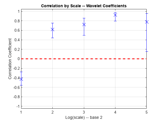
Personal expenditure and personal investment are negatively correlated over a period of 2-4 quarters. At longer scales, there is a strong positive correlation between personal expenditure and personal investment. Examine the wavelet cross-correlation sequence at the scale representing 2-4 quarter cycles. Plot the cross-correlation sequence along with 95% confidence intervals.
[xcseq,xcseqci,lags] = modwtxcorr(piwt,pcwt,'fk8');
zerolag = floor(numel(xcseq{1})/2)+1;
figure
plot(lags{1}(zerolag:zerolag+20),xcseq{1}(zerolag:zerolag+20))
hold on
plot(lags{1}(zerolag:zerolag+20),xcseqci{1}(zerolag:zerolag+20,:),'r--')
xlabel('Lag (Quarters)')
ylabel('Cross-Correlation')
grid on
title({'Wavelet Cross-Correlation Sequence -- [2Q,4Q)'; ...
    'Personal Consumption and Private Investment'})

The finest-scale wavelet cross-correlation sequence shows a peak positive correlation at a lag of one quarter. This indicates that personal investment lags personal expenditures by one quarter. If you take that lagging relationship into account, then there is a positive correlation between the GDP components at all scales.