연속 웨이블릿 변환으로부터 특정 주파수나 시간으로 국소화하여 복원
고베 지진 데이터를 특정 주파수로 국소화하여 근사 성분을 복원합니다. 데이터는 1Hz로 샘플링됩니다. CWT에서 [0.030, 0.070]Hz 주파수 범위에 있는 정보를 추출합니다.
load kobe
Fs = 1;
데이터의 CWT를 구합니다.
[wt,f] = cwt(kobe,Fs);
변환된 데이터에 다시 신호 평균을 더하여 지진 데이터를 복원합니다.
xrec = icwt(wt,[],f,[0.030 0.070],SignalMean=mean(kobe));
원본 데이터와 [0.030, 0.070]Hz 주파수 범위에 있는 데이터를 플로팅하고 비교합니다.
t = (0:numel(kobe)-1)/60;
tiledlayout(2,1)
nexttile
plot(t,kobe)
grid on
title("Original Data")
nexttile
plot(t,xrec)
grid on
xlabel("Time (mins)")
title("Bandpass Filtered Reconstruction [0.030 0.070] Hz")
![Figure contains 2 axes objects. Axes object 1 with title Original Data contains an object of type line. Axes object 2 with title Bandpass Filtered Reconstruction [0.030 0.070] Hz, xlabel Time (mins) contains an object of type line.](../../examples/wavelet/win64/cwtftdemo_01.png)
CWT에 주파수 대신 시간 주기를 사용할 수도 있습니다. 매월 샘플링된 엘니뇨 데이터를 불러옵니다. 시간 주기를 연 단위로 지정하여 데이터의 CWT를 구합니다.
load ninoairdata
[cfs,period] = cwt(nino,years(1/12));
2년부터 8년까지의 역 CWT를 구합니다.
xrec = icwt(cfs,[],period,[years(2) years(8)]);
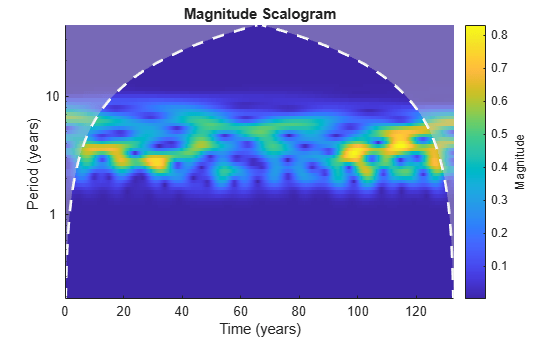
복원된 데이터의 CWT를 플로팅합니다. 2년부터 8년 사이의 대역을 벗어난 영역에는 에너지가 없는 것을 볼 수 있습니다.
figure
cwt(xrec,years(1/12))
원래 데이터와 2년부터 8년까지의 복원 데이터를 비교합니다.
figure
tiledlayout(2,1)
nexttile
plot(datayear,nino)
grid on
title("Original Data")
nexttile
plot(datayear,xrec)
grid on
title("El Nino Data - Years 2-8")
