sheart2
Shearlet transform
Syntax
Description
coefs = sheart2(sls,im)im for the shearlet system sls. If the shearlet
system is real-valued with periodic boundary conditions, then coefs is
real-valued. Otherwise, coefs is complex-valued. The size and class
(data type) of im must match the ImageSize and
Precision
values, respectively, of sls.
Examples
This example shows how to take the shearlet transform of an image and reconstruct the image using only coefficients corresponding to zero shearing.
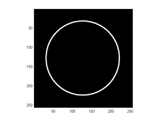
Load and display an image of a circle.
load circleGS
imagesc(circleGS)
colormap gray
axis equal
axis tight
Create a shearlet system that can be used with the image. Obtain the shearlet filters defined by the system, as well as their geometric interpretations.
[numRows,numCols] = size(circleGS);
sls = shearletSystem('ImageSize',[numRows numCols], ...
    'FilterBoundary','truncated');
[psi,scale,shear,cone] = filterbank(sls);
Obtain the shearlet transform of the image.
cfs = sheart2(sls,circleGS);
Find the indices of the shearlet filters that correspond to zero shearing. Keep in mind that the lowpass filter also corresponds to zero shearing.
ind = find((shear==0).*(scale~=-1))'
ind = 1×10

     3     6    10    15    20    25    31    38    46    55
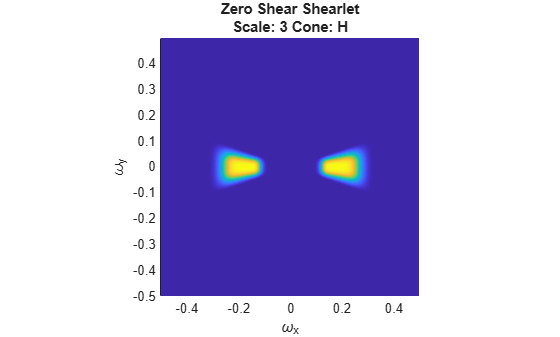
Plot one of the shearlets in the frequency plane. Because the shearlet corresponds to zero shearing, confirm the frequency response is concentrated along either the horizontal or vertical axis.
sh = 31;
omegax = -1/2:1/numCols:1/2-1/numCols;
omegay = omegax;
figure
surf(omegax,flip(omegay),psi(:,:,sh),'EdgeColor','none')
view(0,90)
xlabel('\omega_x')
ylabel('\omega_y')
axis equal
axis tight
title({"Zero Shear Shearlet", ...
    "Scale: "+num2str(scale(sh))+" Cone: "+cone{sh}})
Create an array that only contains the shearlet coefficients that correspond to the zero shearing filters.
cfsx = zeros(size(cfs));
for k=1:length(ind)
    cfsx(:,:,ind(k)) = cfs(:,:,ind(k));
end
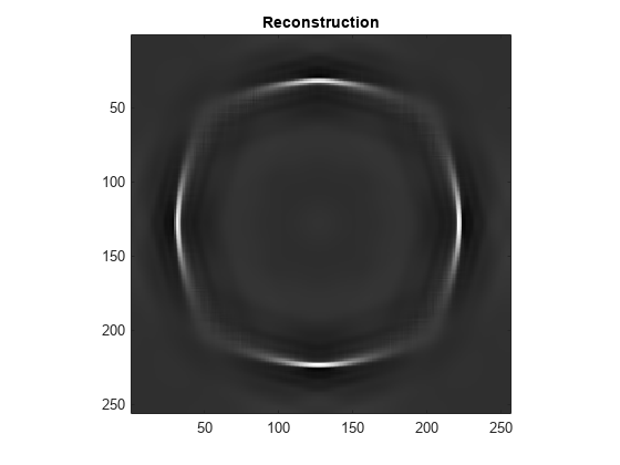
Reconstruct the image using the new coefficients array. Because the only nonzero shearlet coefficients are those that correspond to zero shearing, the horizontal and vertical portions of the circle are emphasized in the reconstruction.
rec = isheart2(sls,cfsx);
imagesc(rec)
axis equal
axis tight
colormap gray
title('Reconstruction')
Input Arguments
Output Arguments
Extended Capabilities
Version History
Introduced in R2019b