bernstein

Bernstein polynomials

Syntax

bernstein(f,n,t)

bernstein(g,n,t)

bernstein(g,var,n,t)

Description

bernstein(f,n,t) with a function handle f returns the nth-order Bernstein polynomial symsum(nchoosek(n,k)*t^k*(1-t)^(n-k)*f(k/n),k,0,n), evaluated at the point t. This polynomial approximates the function f over the interval [0,1].

bernstein(g,n,t) with a symbolic expression or function g returns the nth-order Bernstein polynomial, evaluated at the point t. This syntax regards g as a univariate function of the variable determined by symvar(g,1).

If any argument is symbolic, bernstein converts all arguments except a function handle to symbolic, and converts a function handle’s results to symbolic.

bernstein(g,var,n,t) with a symbolic expression or function g returns the approximating nth-order Bernstein polynomial, regarding g as a univariate function of the variable var.

Examples

Approximation of Sine Function Specified as Function Handle

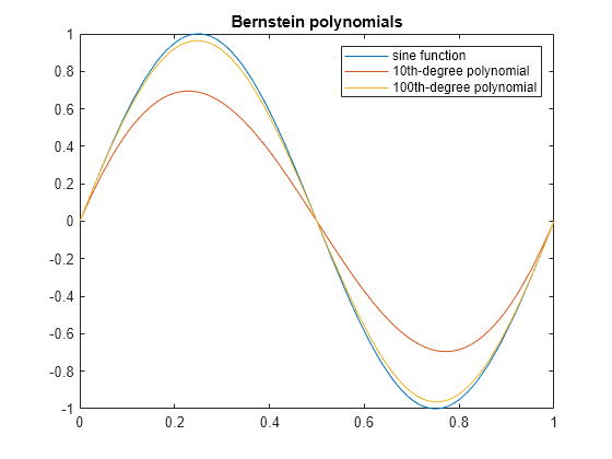
Approximate the sine function by the 10th- and 100th-degree Bernstein polynomials.

syms t
b10 = bernstein(@(t) sin(2*pi*t), 10, t);
b100 = bernstein(@(t) sin(2*pi*t), 100, t);

Plot sin(2*pi*t) and its approximations.

fplot(sin(2*pi*t),[0,1])
hold on
fplot(b10,[0,1])
fplot(b100,[0,1])

legend('sine function','10th-degree polynomial',...
                      '100th-degree polynomial')
title('Bernstein polynomials')
hold off

Approximation of Exponential Function Specified as Symbolic Expression

Approximate the exponential function by the second-order Bernstein polynomial in the variable t:

syms x t
bernstein(exp(x), 2, t)

ans =
(t - 1)^2 + t^2*exp(1) - 2*t*exp(1/2)*(t - 1)

Approximate the multivariate exponential function. When you approximate a multivariate function, bernstein regards it as a univariate function of the default variable determined by symvar. The default variable for the expression y*exp(x*y) is x:

syms x y t
symvar(y*exp(x*y), 1)

ans =
x

bernstein treats this expression as a univariate function of x:

bernstein(y*exp(x*y), 2, t)

ans =
y*(t - 1)^2 + t^2*y*exp(y) - 2*t*y*exp(y/2)*(t - 1)

To treat y*exp(x*y) as a function of the variable y, specify the variable explicitly:

bernstein(y*exp(x*y), y, 2, t)

ans =
t^2*exp(x) - t*exp(x/2)*(t - 1)

Approximation of Linear Ramp Specified as Symbolic Function

Approximate function f representing a linear ramp by the fifth-order Bernstein polynomials in the variable t:

syms f(t)
f(t) = triangularPulse(1/4, 3/4, Inf, t);
p = bernstein(f, 5, t)

p =
7*t^3*(t - 1)^2 - 3*t^2*(t - 1)^3 - 5*t^4*(t - 1) + t^5

Simplify the result:

simplify(p)

ans =
-t^2*(2*t - 3)

Numerical Stability of Simplified Bernstein Polynomials

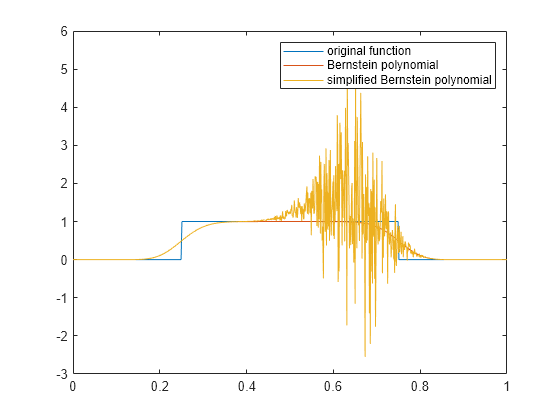
When you simplify a high-order symbolic Bernstein polynomial, the result often cannot be evaluated in a numerically stable way.

Approximate this rectangular pulse function by the 100th-degree Bernstein polynomial, and then simplify the result.

f = @(x)rectangularPulse(1/4,3/4,x);
b1 = bernstein(f, 100, sym('t'));
b2 = simplify(b1);

Convert the polynomial b1 and the simplified polynomial b2 to MATLAB® functions.

f1 = matlabFunction(b1);
f2 = matlabFunction(b2);

Compare the plot of the original rectangular pulse function, its numerically stable Bernstein representation f1, and its simplified version f2. The simplified version is not numerically stable.

t = 0:0.001:1;
plot(t, f(t), t, f1(t), t, f2(t))
hold on
legend('original function','Bernstein polynomial',...
                'simplified Bernstein polynomial')
hold off

Input Arguments

f — Function to be approximated by a polynomial

function handle

Function to be approximated by a polynomial, specified as a function handle. f must accept one scalar input argument and return a scalar value.

g — Function to be approximated by a polynomial

symbolic expression | symbolic function

Function to be approximated by a polynomial, specified as a symbolic expression or function.

n — Bernstein polynomial order

nonnegative integer

Bernstein polynomial order, specified as a nonnegative number.

t — Evaluation point

number | symbolic number | symbolic variable | symbolic expression | symbolic function

Evaluation point, specified as a number, symbolic number, variable, expression, or function. If t is a symbolic function, the evaluation point is the mathematical expression that defines t. To extract the mathematical expression defining t, bernstein uses formula(t).

var — Free variable

symbolic variable

Free variable, specified as a symbolic variable.

More About

Bernstein Polynomials

A Bernstein polynomial is a linear combination of Bernstein basis polynomials.

A Bernstein polynomial of degree n is defined as follows:

$$B\left(t\right)={\displaystyle \sum _{k=0}^n{\beta }_k{b}_{k,n}\left(t\right)}.$$

Here,

$$b_{k,n}\left(t\right)=\left(\begin{array}{c}n\\ k\end{array}\right)t^k{\left(1-t\right)}^{n-k},k=0,\dots ,n$$

are the Bernstein basis polynomials, and $$\left(\begin{array}{c}n\\ k\end{array}\right)$$ is a binomial coefficient.

The coefficients $${\beta }_k$$ are called Bernstein coefficients or Bezier coefficients.

If f is a continuous function on the interval [0, 1] and

$$B_n\left(f\right)\left(t\right)={\displaystyle \sum _{k=0}^{n}f\left(\frac{k}{n}\right)b_{k,n}\left(t\right)}$$

is the approximating Bernstein polynomial, then

$$\underset{n\to \infty }{\lim }{B}_n\left(f\right)\left(t\right)=f\left(t\right)$$

uniformly in t on the interval [0, 1].

Tips

• Symbolic polynomials returned for symbolic t are numerically stable when substituting numerical values between 0 and 1 for t.

• If you simplify a symbolic Bernstein polynomial, the result can be unstable when substituting numerical values for the curve parameter t.

Version History

Introduced in R2013b