Ridge Regression
Introduction to Ridge Regression
Coefficient estimates for the models described in Linear Regression rely on the independence of the model terms. When terms are correlated and the columns of the design matrix X have an approximate linear dependence, the matrix (XTX)–1 becomes close to singular. As a result, the least-squares estimate
becomes highly sensitive to random errors in the observed response y, producing a large variance. This situation of multicollinearity can arise, for example, when data are collected without an experimental design.
Ridge regression addresses the problem by estimating regression coefficients using
where k is the ridge parameter and I is the identity matrix. Small positive values of k improve the conditioning of the problem and reduce the variance of the estimates. While biased, the reduced variance of ridge estimates often result in a smaller mean squared error when compared to least-squares estimates.
The Statistics and Machine Learning Toolbox™ function ridge carries out ridge regression.
Ridge Regression
This example shows how to perform ridge regression.
Load the data in acetylene.mat, with observations of the predictor variables x1, x2, x3, and the response variable y.
load acetylenePlot the predictor variables against each other.
subplot(1,3,1)
plot(x1,x2,'.')
xlabel('x1')
ylabel('x2')
grid on
axis square

subplot(1,3,2)
plot(x1,x3,'.')
xlabel('x1')
ylabel('x3')
grid on
axis square

subplot(1,3,3)
plot(x2,x3,'.')
xlabel('x2')
ylabel('x3')
grid on
axis square
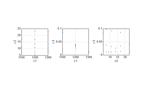
Note the correlation between x1 and the other two predictor variables.
Use ridge and x2fx to compute coefficient estimates for a multilinear model with interaction terms, for a range of ridge parameters.
X = [x1 x2 x3];
D = x2fx(X,'interaction');
D(:,1) = []; % No constant term
k = 0:1e-5:5e-3;
betahat = ridge(y,D,k);
Plot the ridge trace.
figure
plot(k,betahat,'LineWidth',2)
ylim([-100 100])
grid on
xlabel('Ridge Parameter')
ylabel('Standardized Coefficient')
title('{\bf Ridge Trace}')
legend('x1','x2','x3','x1x2','x1x3','x2x3')
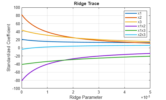
The estimates stabilize to the right of the plot. Note that the coefficient of the x2x3 interaction term changes sign at a value of the ridge parameter .
See Also
lasso | lassoglm | fitrlinear | lassoPlot | ridge