Longitudinal Analysis

This example shows how to perform longitudinal analysis using mvregress.

Load sample data.
Plot data.
Define design matrices.
Fit the model.
Plot fitted model.
Define a reduced model.
Fit the reduced model.
Conduct a likelihood ratio test.

Load sample data.

Load the sample longitudinal data.

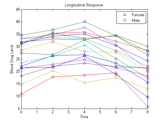
load longitudinalData

The matrix Y contains response data for 16 individuals. The response is the blood level of a drug measured at five time points (t = 0, 2, 4, 6, and 8). Each row of Y corresponds to an individual, and each column corresponds to a time point. The first eight subjects are female, and the second eight subjects are male. This is simulated data.

Plot data.

Plot the data for all 16 subjects.

figure()
t = [0,2,4,6,8];
plot(t,Y)
hold on

hf = plot(t,Y(1:8,:),'^');
hm = plot(t,Y(9:16,:),'o');
legend([hf(1),hm(1)],'Female','Male','Location','NorthEast')

title('Longitudinal Response')
ylabel('Blood Drug Level')
xlabel('Time')
hold off

Blood drug level for 16 subjects at time points 0, 2, 4, 6, and 8. Triangle markers indicate values for female subjects, and circle markers indicate values for male subjects.

Define design matrices.

Let y_ij denote the response for individual i = 1,...,n measured at times t_ij, j = 1,...,d. In this example, n = 16 and d = 5. Let G_i denote the gender of individual i, where G_i = 1 for males and 0 for females.

Consider fitting a quadratic longitudinal model, with a separate slope and intercept for each gender,

$y_{i j} = β_{0} + β_{1} G_{i} + β_{2} t_{i j} + β_{3} t_{i j}^{2} + β_{4} G_{i} \times t_{i j} + β_{5} G_{i} \times t_{i j}^{2} + ε_{i j},$

where $ε_{i} = (ε_{i 1}, \dots, ε_{i d})^{'} \sim M V N (0, Σ)$ . The error correlation accounts for clustering within an individual.

To fit this model using mvregress, the response data should be in an n-by-d matrix. Y is already in the proper format.

Next, create a length-n cell array of d-by-K design matrices. For this model, there are K = 6 parameters.

For individual i, the 5-by-6 design matrix is

$X {i} = (\begin{matrix} 1 & G_{i} & t_{i 1} & t_{i 1}^{2} & G_{i} \times t_{i 1} & G_{i} \times t_{i 1}^{2} \\ 1 & G_{i} & t_{i 2} & t_{i 2}^{2} & G_{i} \times t_{i 2} & G_{i} \times t_{i 2}^{2} \\ ⋮ & ⋮ & ⋮ & ⋮ & ⋮ & ⋮ \\ 1 & G_{i} & t_{i 5} & t_{i 5}^{2} & G_{i} \times t_{i 5} & G_{i} \times t_{i 5}^{2} \end{matrix}),$

corresponding to the parameter vector

$β = (\begin{array}{l} β_{0} \\ β_{1} \\ ⋮ \\ β_{5} \end{array}) .$

The matrix X1 has the design matrix for a female, and X2 has the design matrix for a male.

Create a cell array of design matrices. The first eight individuals are females, and the second eight are males.

X = cell(8,1);
X(1:8) = {X1};
X(9:16) = {X2};

Fit the model.

Fit the model using maximum likelihood estimation. Display the estimated coefficients and standard errors.

[b,sig,E,V,loglikF] = mvregress(X,Y);
[b sqrt(diag(V))]

ans =

   18.8619    0.7432
   13.0942    1.0511
    2.5968    0.2845
   -0.3771    0.0398
   -0.5929    0.4023
    0.0290    0.0563

The coefficients on the interaction terms (in the last two rows of b) do not appear significant. You can use the value of the loglikelihood objective function for this fit, loglikF, to compare this model to one without the interaction terms using a likelihood ratio test.

Plot fitted model.

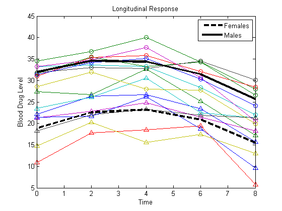
Plot the fitted lines for females and males.

Yhatf = X1*b;
Yhatm = X2*b;

figure()
plot(t,Y)
hold on

plot(t,Y(1:8,:),'^',t,Y(9:16,:),'o')

hf = plot(t,Yhatf,'k--','LineWidth',3);
hm = plot(t,Yhatm,'k','LineWidth',3);
legend([hf,hm],'Females','Males','Location','NorthEast')

title('Longitudinal Response')
ylabel('Blood Drug Level')
xlabel('Time')
hold off

Fitted lines for female and male subjects, which are dotted and solid, respectively

Define a reduced model.

Fit the model without interaction terms,

$y_{i j} = β_{0} + β_{1} G_{i} + β_{2} t_{i j} + β_{3} t_{i j}^{2} + ε_{i j},$

where $ε_{i} = (ε_{i 1}, \dots, ε_{i d})^{'} \sim M V N (0, Σ)$ .

This model has four coefficients, which correspond to the first four columns of the design matrices X1 and X2 (for females and males, respectively).

X1R = X1(:,1:4);
X2R = X2(:,1:4);

XR = cell(8,1);
XR(1:8) = {X1R};
XR(9:16) = {X2R};

Fit the reduced model.

Fit this model using maximum likelihood estimation. Display the estimated coefficients and their standard errors.

[bR,sigR,ER,VR,loglikR] = mvregress(XR,Y);
[bR,sqrt(diag(VR))]

ans =

   19.3765    0.6898
   12.0936    0.8591
    2.2919    0.2139
   -0.3623    0.0283

Conduct a likelihood ratio test.

Compare the two models using a likelihood ratio test. The null hypothesis is that the reduced model is sufficient. The alternative is that the reduced model is inadequate (compared to the full model with the interaction terms).

The likelihood ratio test statistic is compared to a chi-squared distribution with two degrees of freedom (for the two coefficients being dropped).

LR = 2*(loglikF-loglikR);
pval = 1 - chi2cdf(LR,2)

pval =

    0.0803

The p-value 0.0803 indicates that the null hypothesis is not rejected at the 5% significance level. Therefore, there is insufficient evidence that the extra terms improve the fit.