response
Class: GeneralizedLinearMixedModel
Response vector of generalized linear mixed-effects model
Description
Input Arguments
Output Arguments
Examples
Load the sample data.
load mfrThis simulated data is from a manufacturing company that operates 50 factories across the world, with each factory running a batch process to create a finished product. The company wants to decrease the number of defects in each batch, so it developed a new manufacturing process. To test the effectiveness of the new process, the company selected 20 of its factories at random to participate in an experiment: Ten factories implemented the new process, while the other ten continued to run the old process. In each of the 20 factories, the company ran five batches (for a total of 100 batches) and recorded the following data:
Flag to indicate whether the batch used the new process (
newprocess)Processing time for each batch, in hours (
time)Temperature of the batch, in degrees Celsius (
temp)Categorical variable indicating the supplier (
A,B, orC) of the chemical used in the batch (supplier)Number of defects in the batch (
defects)
The data also includes time_dev and temp_dev, which represent the absolute deviation of time and temperature, respectively, from the process standard of 3 hours at 20 degrees Celsius.
Fit a generalized linear mixed-effects model using newprocess, time_dev, temp_dev, and supplier as fixed-effects predictors. Include a random-effects term for intercept grouped by factory, to account for quality differences that might exist due to factory-specific variations. The response variable defects has a Poisson distribution, and the appropriate link function for this model is log. Use the Laplace fit method to estimate the coefficients. Specify the dummy variable encoding as 'effects', so the dummy variable coefficients sum to 0.
The number of defects can be modeled using a Poisson distribution
This corresponds to the generalized linear mixed-effects model
where
is the number of defects observed in the batch produced by factory during batch .
is the mean number of defects corresponding to factory (where ) during batch (where ).
, , and are the measurements for each variable that correspond to factory during batch . For example, indicates whether the batch produced by factory during batch used the new process.
and are dummy variables that use effects (sum-to-zero) coding to indicate whether company
CorB, respectively, supplied the process chemicals for the batch produced by factory during batch .is a random-effects intercept for each factory that accounts for factory-specific variation in quality.
glme = fitglme(mfr,'defects ~ 1 + newprocess + time_dev + temp_dev + supplier + (1|factory)',...
    'Distribution','Poisson','Link','log','FitMethod','Laplace','DummyVarCoding','effects');
Extract the observed response values for the model, then use fitted to generate the fitted conditional mean values.
y = response(glme);   % Observed response values
yfit = fitted(glme);  % Fitted response values
Create a scatterplot of the observed response values versus fitted values. Add a reference line to improve the visualization.
figure
scatter(yfit,y)
xlim([0,12])
ylim([0,12])
refline(1,0)
title('Response versus Fitted Values')
xlabel('Fitted Values')
ylabel('Response')
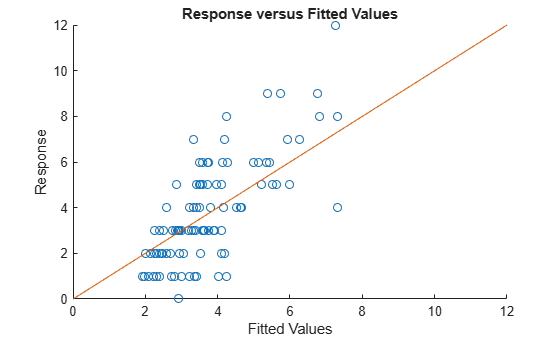
The plot shows a positive correlation between the fitted values and the observed response values.
References
[1] Hox, J. Multilevel Analysis, Techniques and Applications. Lawrence Erlbaum Associates, Inc., 2002.