disparateImpactRemover
Description
To try to create fairness in binary classification, you can use the
disparateImpactRemover function to remove or reduce the disparate
impact of a sensitive attribute. Before training your model, use the sensitive attribute to
transform the continuous predictors in the training data set. The function returns the
transformed data set and a disparateImpactRemover object that contains the
transformation. Pass the transformed data set to an appropriate training function, such as
fitcsvm, and pass the object to the transform object
function to apply the transformation to a new data set, such as a test data
set.
Note
You must transform new data, such as test data, after training a model using
disparateImpactRemover. Otherwise, the predicted results are
inaccurate.
Creation
Syntax
Description
remover = disparateImpactRemover(Tbl,AttributeName)AttributeName sensitive attribute
in the table Tbl by transforming the continuous predictors in the
data set Tbl. The returned disparateImpactRemover
object (remover) stores the transformation, which you can apply to
new data. For more information, see Algorithms.
[
also returns the transformed predictor data remover,transformedData] = disparateImpactRemover(Tbl,AttributeName)transformedData, which
corresponds to the data in Tbl.
Note that transformedData includes the sensitive attribute in
this syntax. After using disparateImpactRemover, avoid using the
sensitive attribute as a separate predictor when training your model.
[
uses the numeric predictor data remover,transformedData] = disparateImpactRemover(X,attribute)X and the sensitive attribute
specified by attribute to transform the predictors.
[
specifies options using one or more name-value arguments in addition to any of the input
argument combinations in previous syntaxes. For example, you can specify the extent of the
data transformation by using the remover,transformedData] = disparateImpactRemover(___,Name=Value)RepairFraction name-value argument.
A value of 1 indicates a full transformation, and a value of 0 indicates no
transformation.
Input Arguments
Name-Value Arguments
Output Arguments
Properties
Object Functions
transform | Transform new predictor data to remove disparate impact |
Examples
Train a binary classifier, classify test data using the model, and compute the disparate impact for each group in the sensitive attribute. To reduce the disparate impact values, use disparateImpactRemover, and then retrain the binary classifier. Transform the test data set, reclassify the observations, and compute the disparate impact values.
Load the sample data census1994, which contains the training data adultdata and the test data adulttest. The data sets consist of demographic information from the US Census Bureau that can be used to predict whether an individual makes over $50,000 per year. Preview the first few rows of the training data set.
load census1994
head(adultdata)
age workClass fnlwgt education education_num marital_status occupation relationship race sex capital_gain capital_loss hours_per_week native_country salary
___ ________________ __________ _________ _____________ _____________________ _________________ _____________ _____ ______ ____________ ____________ ______________ ______________ ______
39 State-gov 77516 Bachelors 13 Never-married Adm-clerical Not-in-family White Male 2174 0 40 United-States <=50K
50 Self-emp-not-inc 83311 Bachelors 13 Married-civ-spouse Exec-managerial Husband White Male 0 0 13 United-States <=50K
38 Private 2.1565e+05 HS-grad 9 Divorced Handlers-cleaners Not-in-family White Male 0 0 40 United-States <=50K
53 Private 2.3472e+05 11th 7 Married-civ-spouse Handlers-cleaners Husband Black Male 0 0 40 United-States <=50K
28 Private 3.3841e+05 Bachelors 13 Married-civ-spouse Prof-specialty Wife Black Female 0 0 40 Cuba <=50K
37 Private 2.8458e+05 Masters 14 Married-civ-spouse Exec-managerial Wife White Female 0 0 40 United-States <=50K
49 Private 1.6019e+05 9th 5 Married-spouse-absent Other-service Not-in-family Black Female 0 0 16 Jamaica <=50K
52 Self-emp-not-inc 2.0964e+05 HS-grad 9 Married-civ-spouse Exec-managerial Husband White Male 0 0 45 United-States >50K
Each row contains the demographic information for one adult. The last column salary shows whether a person has a salary less than or equal to $50,000 per year or greater than $50,000 per year.
Remove observations from adultdata and adulttest that contain missing values.
adultdata = rmmissing(adultdata);
adulttest = rmmissing(adulttest);
Specify the continuous numeric predictors to use for model training.
predictors = ["age","education_num","capital_gain","capital_loss", ...
    "hours_per_week"];
Train an ensemble classifier using the training set adultdata. Specify salary as the response variable and fnlwgt as the observation weights. Because the training set is imbalanced, use the RUSBoost algorithm. After training the model, predict the salary (class label) of the observations in the test set adulttest.
rng("default") % For reproducibility
mdl = fitcensemble(adultdata,"salary",Weights="fnlwgt", ...
    PredictorNames=predictors,Method="RUSBoost");
labels = predict(mdl,adulttest);
Transform the training set predictors by using the race sensitive attribute.
[remover,newadultdata] = disparateImpactRemover(adultdata, ...
    "race",PredictorNames=predictors);
remover
remover =
  disparateImpactRemover with properties:

        RepairFraction: 1
        PredictorNames: {'age'  'education_num'  'capital_gain'  'capital_loss'  'hours_per_week'}
    SensitiveAttribute: 'race'
remover is a disparateImpactRemover object, which contains the transformation of the remover.PredictorNames predictors with respect to the remover.SensitiveAttribute variable.
Apply the same transformation stored in remover to the test set predictors. Note: You must transform both the training and test data sets before passing them to a classifier.
newadulttest = transform(remover,adulttest, ...
    PredictorNames=predictors);
Train the same type of ensemble classifier as mdl, but use the transformed predictor data. As before, predict the salary (class label) of the observations in the test set adulttest.
rng("default") % For reproducibility
newMdl = fitcensemble(newadultdata,"salary",Weights="fnlwgt", ...
    PredictorNames=predictors,Method="RUSBoost");
newLabels = predict(newMdl,newadulttest);
Compare the disparate impact values for the predictions made by the original model (mdl) and the predictions made by the model trained with the transformed data (newMdl). For each group in the sensitive attribute, the disparate impact value is the proportion of predictions in that group with a positive class value () divided by the proportion of predictions in the reference group with a positive class value (). An ideal classifier makes predictions where, for each group, is close to (that is, where the disparate impact value is close to 1).
Compute the disparate impact values for the mdl predictions and the newMdl predictions by using fairnessMetrics. Include the observation weights. You can use the report object function to display bias metrics, such as disparate impact, that are stored in the metricsResults object.
metricsResults = fairnessMetrics(adulttest,"salary", ...
    SensitiveAttributeNames="race",Predictions=[labels,newLabels], ...
    Weights="fnlwgt",ModelNames=["Original Model","New Model"]);
metricsResults.PositiveClass
ans = categorical
     >50K
metricsResults.ReferenceGroup
ans =
'White'
report(metricsResults,BiasMetrics="DisparateImpact")ans=5×5 table
Metrics SensitiveAttributeNames Groups Original Model New Model
_______________ _______________________ __________________ ______________ _________
DisparateImpact race Amer-Indian-Eskimo 0.41702 0.92804
DisparateImpact race Asian-Pac-Islander 1.719 0.9697
DisparateImpact race Black 0.60571 0.66629
DisparateImpact race Other 0.66958 0.86039
DisparateImpact race White 1 1
For the mdl predictions, several of the disparate impact values are below the industry standard of 0.8, and one value is above 1.25. These values indicate bias in the predictions with respect to the positive class >50K and the sensitive attribute race.
The disparate impact values for the newMdl predictions are closer to 1 than the disparate impact values for the mdl predictions. One value is still below 0.8.
Visually compare the disparate impact values by using the bar graph returned by the plot object function.
plot(metricsResults,"DisparateImpact")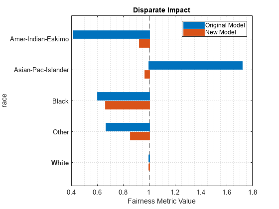
The disparateImpactRemover function seems to have improved the model predictions on the test set with respect to the disparate impact metric.
Check whether the transformed predictors negatively affect the accuracy of the model predictions. Compute the accuracy of the test set predictions for the two models mdl and newMdl.
accuracy = 1-loss(mdl,adulttest,"salary")accuracy = 0.8024
newAccuracy = 1-loss(newMdl,newadulttest,"salary")newAccuracy = 0.7955
The model trained using the transformed predictors (newMdl) achieves similar test set accuracy compared to the model trained with the original predictors (mdl).
Try to remove the disparate impact of a sensitive attribute by adjusting continuous numeric predictors. Visualize the difference between the original and adjusted predictor values.
Suppose you want to create a binary classifier that predicts whether a patient is a smoker based on the patient's diastolic and systolic blood pressure values. Also, you want to remove the disparate impact of the patient's gender on model predictions. Before training the model, you can use disparateImpactRemover to transform the continuous predictor variables in your data set.
Load the patients data set, which contains medical information for 100 patients. Convert the Gender and Smoker variables to categorical variables. Specify the descriptive category names Smoker and Nonsmoker rather than 1 and 0.
load patients
Gender = categorical(Gender);
Smoker = categorical(Smoker,logical([1 0]), ...
    ["Smoker","Nonsmoker"]);
Create a matrix containing the continuous predictors Diastolic and Systolic.
X = [Diastolic,Systolic];
Find the observations in the two groups of the sensitive attribute Gender.
femaleIdx = Gender=="Female";
maleIdx = Gender=="Male";
femaleX = X(femaleIdx,:);
maleX = X(maleIdx,:);
Compute the Diastolic and Systolic quantiles for the two groups in the sensitive attribute. Specify the number of quantiles to be the minimum number of group observations across the groups in the sensitive attribute, provided that the number is smaller than 100.
t = tabulate(Gender);
t = array2table(t,VariableNames=["Value","Count","Percent"])
t=2×3 table
      Value       Count     Percent
    __________    ______    _______

    {'Female'}    {[53]}    {[53]}
    {'Male'  }    {[47]}    {[47]}
numQuantiles = min(100,min(t.Count{:}))numQuantiles = 47
femaleQuantiles = quantile(femaleX,numQuantiles,1);
maleQuantiles = quantile(maleX,numQuantiles,1);
Compute the median quantiles across the two groups.
Q(:,:,1) = femaleQuantiles;
Q(:,:,2) = maleQuantiles;
medianQuantiles = median(Q,3);
Plot the results. Show the Diastolic quantiles in the left plot and the Systolic quantiles in the right plot.
tiledlayout(1,2)

nexttile % Diastolic
plot(femaleQuantiles(:,1),1:numQuantiles)
hold on
plot(maleQuantiles(:,1),1:numQuantiles)
plot(medianQuantiles(:,1),1:numQuantiles)
hold off
xlabel("Diastolic")
ylabel("Quantile")
legend(["Female","Male","Median"],Location="southeast")

nexttile % Systolic
plot(femaleQuantiles(:,2),1:numQuantiles)
hold on
plot(maleQuantiles(:,2),1:numQuantiles)
plot(medianQuantiles(:,2),1:numQuantiles)
hold off
xlabel("Systolic")
ylabel("Quantile")
legend(["Female","Male","Median"],Location="southeast")
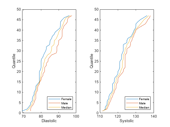
For each predictor, the Female and Male quantiles differ. The disparateImpactRemover function uses the median quantiles to adjust this difference.
Transform the Diastolic and Systolic predictors in X by using the Gender sensitive attribute.
[remover,newX] = disparateImpactRemover(X,Gender);
femaleNewX = newX(femaleIdx,:);
maleNewX = newX(maleIdx,:);
Visualize the difference in the Diastolic distributions between the original values in X and the transformed values in newX. Compute and display the probability density estimates by using the ksdensity function.
tiledlayout(1,2)

nexttile
ksdensity(femaleX(:,1))
hold on
ksdensity(maleX(:,1))
hold off
xlabel("Diastolic")
ylabel("Probability Density Estimate")
title("Original")
legend(["Female","Male"])
ylim([0,0.07])

nexttile
ksdensity(femaleNewX{:,1})
hold on
ksdensity(maleNewX{:,1})
hold off
xlabel("Diastolic")
ylabel("Probability Density Estimate")
title("Transformed")
legend(["Female","Male"])
ylim([0,0.07])
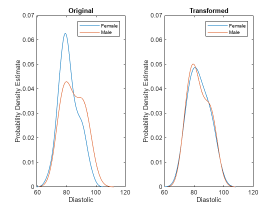
The disparateImpactRemover function transforms the values in the Diastolic predictor variable so that the distribution of Female values and the distribution of Male values are similar.
You can now train a binary classifier using the adjusted predictor data. For this example, train a tree classifier.
tree = fitctree(newX,Smoker)
tree =
  ClassificationTree
           PredictorNames: {'x1'  'x2'}
             ResponseName: 'Y'
    CategoricalPredictors: []
               ClassNames: [Smoker    Nonsmoker]
           ScoreTransform: 'none'
          NumObservations: 100


  Properties, Methods
Note: You must transform new data sets before passing them to the classifier for prediction.
Randomly sample 10 observations from X. Transform the values using the remover object and the transform object function. Then, predict the smoker status for the observations.
rng("default") % For reproducibility
testIdx = randsample(size(X,1),10,1);
testX = transform(remover,X(testIdx,:),Gender(testIdx));
label = predict(tree,testX)
label = 10×1 categorical
     Nonsmoker
     Smoker
     Nonsmoker
     Nonsmoker
     Nonsmoker
     Nonsmoker
     Nonsmoker
     Smoker
     Smoker
     Smoker
Specify the extent of the transformation of the continuous numeric predictors with respect to a sensitive attribute. Use the RepairFraction name-value argument of the disparateImpactRemover function.
Load the patients data set, which contains medical information for 100 patients. Convert the Gender and Smoker variables to categorical variables. Specify the descriptive category names Smoker and Nonsmoker rather than 1 and 0.
load patients
Gender = categorical(Gender);
Smoker = categorical(Smoker,logical([1 0]), ...
    ["Smoker","Nonsmoker"]);
Create a matrix containing the continuous predictors Diastolic and Systolic.
X = [Diastolic,Systolic];
Find the observations in the two groups of the sensitive attribute Gender.
femaleIdx = Gender=="Female";
maleIdx = Gender=="Male";
femaleX = X(femaleIdx,:);
maleX = X(maleIdx,:);
Transform the Diastolic and Systolic predictors in X by using the Gender sensitive attribute. Specify a repair fraction of 0.5. Note that a value of 1 indicates a full transformation, and a value of 0 indicates no transformation.
[remover,newX50] = disparateImpactRemover(X,Gender, ...
    RepairFraction=0.5);
femaleNewX50 = newX50(femaleIdx,:);
maleNewX50 = newX50(maleIdx,:);
Fully transform the predictor variables by using the transform object function of the remover object.
newX100 = transform(remover,X,Gender,RepairFraction=1);
femaleNewX100 = newX100(femaleIdx,:);
maleNewX100 = newX100(maleIdx,:);
Visualize the difference in the Diastolic distributions between the original values in X, the partially repaired values in newX50, and the fully transformed values in newX100. Compute and display the probability density estimates by using the ksdensity function.
t = tiledlayout(1,3);
title(t,"Diastolic Distributions with Different " + ...
    "Repair Fractions")
xlabel(t,"Diastolic")
ylabel(t,"Density Estimate")

nexttile
ksdensity(femaleX(:,1))
hold on
ksdensity(maleX(:,1))
hold off
title("Fraction=0")
ylim([0,0.07])

nexttile
ksdensity(femaleNewX50{:,1})
hold on
ksdensity(maleNewX50{:,1})
hold off
title("Fraction=0.5")
ylim([0,0.07])

nexttile
ksdensity(femaleNewX100{:,1})
hold on
ksdensity(maleNewX100{:,1})
hold off
title("Fraction=1")
ylim([0,0.07])
legend(["Female","Male"],Location="eastoutside")
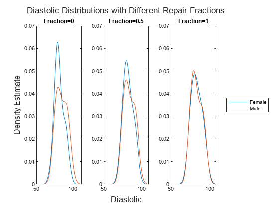
As the repair fraction increases, the disparateImpactRemover function transforms the values in the Diastolic predictor variable so that the distribution of Female values and the distribution of Male values become more similar.
More About
Tips
After using
disparateImpactRemover, consider using only continuous and ordinal predictors for model training. Avoid using the sensitive attribute as a separate predictor when training your model. For more information, see [1].You must transform new data, such as test data, after training a model using
disparateImpactRemover. Otherwise, the predicted results are inaccurate. Use thetransformobject function.
Algorithms
disparateImpactRemover transforms a continuous predictor in
Tbl or X as follows:
The software uses the groups in the sensitive attribute to split the predictor values. For each group g, the software computes q quantiles of the predictor values by using the
quantilefunction. The number of quantiles q is either 100 or the minimum number of group observations across the groups in the sensitive attribute, whichever is smaller. The software creates a corresponding binning function Fg using thediscretizefunction and the quantile values as bin edges.The software then finds the median quantile values across all the sensitive attribute groups and forms the associated quantile function Fm-1. The software omits missing (
NaN) values from this calculation.Finally, the software transforms the predictor value x in the sensitive attribute group g by using the transformation λFm-1(Fg(x)) + (1 – λ)x, where λ is the repair fraction
RepairFraction. The software preserves missing (NaN) values in the predictor.
The function stores the transformation, which you can apply to new predictor data.
For more information, see [1].
References
[1] Feldman, Michael, Sorelle A. Friedler, John Moeller, Carlos Scheidegger, and Suresh Venkatasubramanian. “Certifying and Removing Disparate Impact.” In Proceedings of the 21th ACM SIGKDD International Conference on Knowledge Discovery and Data Mining, 259–68. Sydney NSW Australia: ACM, 2015. https://doi.org/10.1145/2783258.2783311.
Version History
Introduced in R2022b