NPN Bipolar Transistor
NPN bipolar transistor using enhanced Ebers-Moll equations

Libraries:
Simscape /
Electrical /
Semiconductors & Converters
Description
The NPN Bipolar Transistor block uses a variant of the Ebers-Moll equations to represent an NPN bipolar transistor. The Ebers-Moll equations are based on two exponential diodes plus two current-controlled current sources. The NPN Bipolar Transistor block provides these enhancements to that model:
Early voltage effect
Optional base, collector, and emitter resistances
Optional fixed base-emitter and base-collector capacitances
The collector and base currents are:
In these equations:
IB and IC are base and collector currents, defined as positive into the device.
IS is the value of the Saturation current IS parameter.
VBE is the base-emitter voltage and VBC is the base-collector voltage.
βF is the value of the Forward current transfer ratio BF parameter parameter. This term represents the ideal maximum forward current gain.
βR is the value of the Reverse current transfer ratio BR parameter parameter. This term represents the ideal maximum reverse current gain.
VA is the value of the Forward Early voltage VAF parameter.
q is the elementary charge on an electron (1.602176e–19 Coulombs).
k is the Boltzmann constant (1.3806503e–23 J/K).
Tm1 is the transistor temperature, as defined by the Measurement temperature parameter value.
You can specify the transistor behavior using datasheet parameters that the block uses to calculate the parameters for these equations, or you can specify the equation parameters directly.
If qVBC / (kTm1) > 40 or qVBE / (kTm1) > 40, the corresponding exponential terms in the equations are replaced with (qVBC / (kTm1) – 39)e40 and (qVBE / (kTm1) – 39)e40, respectively. This helps prevent numerical issues associated with the steep gradient of the exponential function ex at large values of x. Similarly, if qVBC / (kTm1) < –39 or qVBE / (kTm1) < –39 then the corresponding exponential terms in the equations are replaced with (qVBC / (kTm1) + 40)e–39 and (qVBE / (kTm1) + 40)e–39, respectively.
Optionally, you can specify fixed capacitances across the base-emitter and base-collector junctions. You can also specify base, collector, and emitter connection resistances.
Modeling Capacitance and Charge
You model capacitance and charge using the Base-collector junction capacitance and Base-emitter junction capacitance parameters. You can also represent reverse recovery charge and dynamics using the Total forward transit time and Total reverse transit time parameters. This equation defines the base-collector charge,
where:
tR is the Total reverse transit time parameter value.
ICE is the collector-emitter current.
CBC is the Base-collector junction capacitance parameter value.
VBC is the base-collector voltage.
This equation defines the base-collector charge and capacitor current,
This equation defines base-emitter charge,
where:
tF is the Total forward transit time parameter value.
IC is the collector current.
CBE is the Base-emitter junction capacitance parameter value.
VBE is the base-emitter voltage.
This equation defines the base-emitter charge and capacitor current,
Modeling Temperature Dependence
The default behavior is that dependence on temperature is not modeled, and the device is simulated at the temperature for which you provide block parameters. You can optionally include modeling the dependence of the transistor static behavior on temperature during simulation. Temperature dependence of the junction capacitances is not modeled, this being a much smaller effect.
When including temperature dependence, the transistor defining equations remain the same. The measurement temperature value, Tm1, is replaced with the simulation temperature, Ts. The saturation current, IS, and the forward and reverse gains (βF and βR) become a function of temperature according to the following equations:
where:
Tm1 is the temperature at which the transistor parameters are specified, as defined by the Measurement temperature parameter value.
Ts is the simulation temperature.
ISTm1 is the saturation current at the measurement temperature.
ISTs is the saturation current at the simulation temperature. This is the saturation current value used in the bipolar transistor equations when temperature dependence is modeled.
βFm1 and βRm1 are the forward and reverse gains at the measurement temperature.
βFs and βRs are the forward and reverse gains at the simulation temperature. These are the values used in the bipolar transistor equations when temperature dependence is modeled.
EG is the energy gap for the semiconductor type measured in Joules. The value for silicon is usually taken to be 1.11 eV, where 1 eV is 1.602e-19 Joules.
XTI is the saturation current temperature exponent.
XTB is the forward and reverse gain temperature coefficient.
k is the Boltzmann constant (1.3806503e–23 J/K).
Appropriate values for XTI and EG depend on the type of transistor and the semiconductor material used. In practice, the values of XTI, EG, and XTB need tuning to model the exact behavior of a particular transistor. Some manufacturers quote these tuned values in a SPICE Netlist, and you can read off the appropriate values. Otherwise you can determine values for XTI, EG, and XTB by using a datasheet-defined data at a higher temperature Tm2. The block provides a datasheet parameterization option for this.
You can also tune the values of XTI, EG, and XTB yourself, to match lab data for your particular device. You can use Simulink® Design Optimization™ software to help tune the values.
Thermal Port
You can expose the thermal port to model the effects of generated heat and device temperature. To expose the thermal port, set the Modeling option parameter to either:
No thermal port— The block does not contain a thermal port and does not simulate heat generation in the device.Show thermal port— The block contains a thermal port that allows you to model the heat that conduction losses generate. For numerical efficiency, the thermal state does not affect the electrical behavior of the block.
For more information on using thermal ports and on the Thermal Port parameters, see Simulating Thermal Effects in Semiconductors.
Variables
To set the priority and initial target values for the block variables before simulation, use the Initial Targets section in the block dialog box or Property Inspector. For more information, see Set Priority and Initial Target for Block Variables.
Note
To satisfy all your initial targets, do not set the priority to
High for more initial targets than the total number of
differential variables in the block equations. If you set the Base-collector
junction capacitance or Total reverse transit time
parameter to a nonzero value and set the Base-emitter junction
capacitance or Total forward transit time parameter to a
nonzero value, the number of differential variables in the block equations is two. Choose
one of these options:
To set the terminal current initial condition, in the Initial Targets section, set the priority of only the Base current and Collector current variables to
High.To set the terminal voltage initial condition, in the Initial Targets section, set the priority of only the Collector-emitter voltage and Base-emitter voltage variables to
High.To set the total charge initial condition, in the Initial Targets section, set the priority of only the Base-collector charge and Base-emitter charge variables to
High. (since R2024a)
Use nominal values to specify the expected magnitude of a variable in a model. Using system scaling based on nominal values increases the simulation robustness. Nominal values can come from different sources. One of these sources is the Nominal Values section in the block dialog box or Property Inspector. For more information, see System Scaling by Nominal Values.
Plot Basic I-V Characteristics
You can plot the basic I-V characteristics of the NPN Bipolar Transistor block without building a complete model. Use the plots to explore the impact of your parameter choices on device characteristics. If you parameterize the block from a data sheet, you can compare your plots to the data sheet to check that you parameterized the block correctly. If you have a complete working model but do not know which manufactured part to use, you can compare your plots to data sheets to help you decide.
To plot the basic I-V characteristics, set the Modeling option
parameter to No thermal port and, in the
Utilities section, click the
Plot button next to the Basic
characteristics parameter. (since R2026a) For more information about the
Basic characteristics parameter, see Plot Basic I-V Characteristics of Semiconductor Blocks.
Examples

NPN Bipolar Transistor Characteristics
Generation of the Ic versus Vce curve for an NPN bipolar transistor. Define the vector of base currents and minimum and maximum collector-emitter voltages by double clicking on the block labeled 'Define Conditions (Ib and Vce)'. Run the tests and generate plots of the curves by clicking in the model on hyperlink 'plot curves'.

Linear LED Driver
A LED driver based on a linear current regulator. The scope shows the light and current output and the supply voltage. The output comes into regulation for a supply voltage greater than about 12V.

Linear Voltage Regulator with Feedback
A simple voltage regulator circuit constructed from discrete components. A fluctuating supply is modeled as 20V DC plus a 1V sinusoidal variation. The zener diode D1 sets the non-inverting input of the op-amp to 3.2V, and hence as the op-amp has a large gain, the op-amp inverting input and output are also at 3.2V. Hence the regulator voltage output is regulated to be 3.2*(1000+470)/470=10V. The NPN bipolar transistor is required to provide higher currents than is possible from a typical op-amp. The model can be used to check circuit operation, and to support selection of components to achieve the desired voltage regulation.
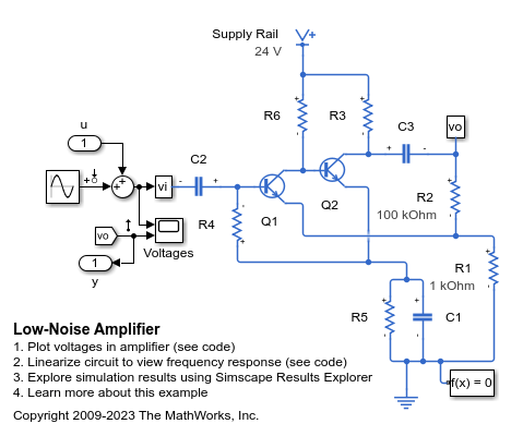
Low-Noise Amplifier
A typical low-noise audio amplifier circuit. Resistor R2 provides negative feedback to stabilize the overall amplifier gain, making it independent of transistor open-loop forward transfer gain. Circuit gain is approximately defined by (R1+R2)/R1 = 101. The simulation shows that it takes the circuit a few seconds to settle to its steady operating point, and that the output is initially clipped. Input u and output y are included to support linearization.
Assumptions and Limitations
The block does not account for temperature-dependent effects on the junction capacitances.
You might need to use nonzero ohmic resistance and junction capacitance values to prevent numerical simulation issues, but the simulation may run faster with these values set to zero.
Ports
The figure shows the block port names.
![]()
Conserving
Parameters
References
[1] G. Massobrio and P. Antognetti. Semiconductor Device Modeling with SPICE. 2nd Edition, McGraw-Hill, 1993.
[2] H. Ahmed and P.J. Spreadbury. Analogue and digital electronics for engineers. 2nd Edition, Cambridge University Press, 1984.