Compute Operating Points Using Custom Constraints and Objective Functions
Typically, when computing a steady-state operating point for a Simulink® model using an optimization-based search, you specify known fixed values or bounds to constrain your model states, inputs, or outputs. However, some systems or applications require additional flexibility in defining the optimization search parameters.
For such systems, you can specify custom constraints, an additional optimization objective function, or both. When the software computes a steady-state operating point, it applies these custom constraints and objective function in addition to the standard state, input, and output specifications.
You can specify custom equality and inequality constraints as algebraic combinations of model states, inputs, and outputs. These constraints let you limit the operating point search space by specifying known relationships between inputs, outputs, and states. For example, you can specify that one model state is the sum of two other states.
You can also specify a custom scalar objective function as an algebraic combination of model states, inputs, and outputs. Using the objective function you can optimize the steady-state operating point based on your application requirements. For example, suppose that your model has multiple potential equilibrium points. You can specify an objective function to find the steady-state point with the minimum input energy.
For complex models, you can specify a custom mapping function that selects a subset of the model inputs, outputs, and states to pass to the custom cost and constraint functions.
You can specify custom optimization functions when trimming your model:
At the command line: Create an operating point specification using
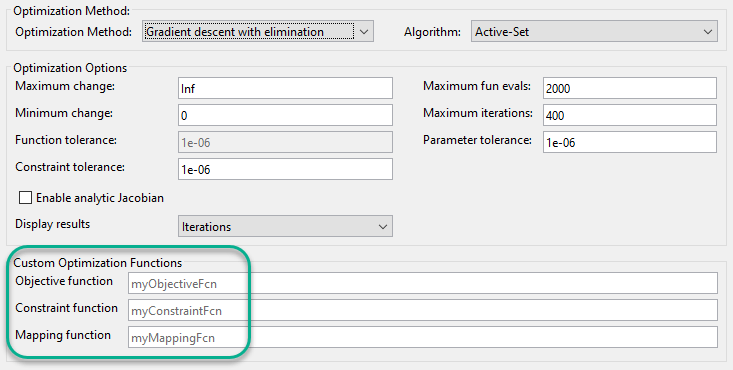
operspec, and specify the custom functions using theCustomConstrFcn,CustomCostFcn, andCustomMappingFcnproperties of the specification.Using the Steady State Manager: On the Specification tab, click Trim Options. In the Trim Options dialog box, in the Custom Optimization Functions section, specify the function names.
Using the Model Linearizer: On the Linear Analysis tab, in the Operating Point drop-down list, click Trim Model. In the Trim the model dialog box, on the Options tab, in the Custom Optimization Functions section, specify the function names.
The following example shows how to create custom optimization functions and how to trim a model at the command line using these custom functions.
Simulink Model
For this example, use a model of three tanks connected with each other by orifices.
mdl = 'scdTanks';
open_system(mdl)
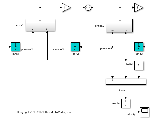
The flow between Tank1 and Tank2 is desired. The flow between Tank2 and Tank3 is undesired unavoidable leakage.
At the expected steady state of this system:
Tank1 and Tank2 have the same pressure.
Tank2 and Tank3 have an almost constant pressure difference of
1that compensates a load.
Due to the weak connectivity between Tank1 and Tank2, it is difficult to trim the model such that the pressures in Tank1 and Tank2 are equal.
Trim Model Without Customizations
Create a default operating point specification for the model. The specification configures all three tank pressures as free states that must be at steady state in the trimmed operating point.
opspec = operspec(mdl);
Create an option set for trimming the model, suppressing the Command Window display of the operating point search report. The specific trimming options depend on your application. For this example, use nonlinear least squares optimization.
opt = findopOptions('OptimizerType','lsqnonlin');
opt.DisplayReport = 'off';
Trim the model, and view the trimmed tank pressures.
[op0,rpt0] = findop(mdl,opspec,opt);
op0.States
ans =

 x
____

(1.) scdTanks/Inertia
 0
(2.) scdTanks/Tank1
 9
(3.) scdTanks/Tank2
9.5
(4.) scdTanks/Tank3
10.5
The trimmed pressures in Tank1 and Tank2 do not match. Thus, the default operating point specification fails to find an operating point that meets the expected steady-state requirements. If you reduce the constraint tolerance, opt.OptimizationOptions.TolCon, you cannot achieve a feasible steady-state solution due to the leakage between Tank2 and Tank3.
Add Custom Constraints
To specify custom constraints, define a function in the current working folder or on the MATLAB® path with input arguments:
x- Operating point specification states, specified as a vector.u- Operating point specification inputs, specified as a vector.y- Operating point specification outputs, specified as a vector.
and output arguments:
c_ineq- Inequality constraints which must satisfyc_ineq <= 0during trimming, returned as a vector.c_eq- Equality constraints which must satisfyc_eq = 0during trimming, returned as a vector.
Each element of c_ineq and c_eq specifies a single constraint. Define the specific constraints for your application as algebraic combinations of the states, inputs, and outputs. If there are no custom equality or inequality constraints, return the corresponding output argument as [].
For this example, to satisfy the conditions of the expected steady state, define the following custom constraint function.
function [c_ineq,c_eq] =  myConstraints(x,u,y)
    c_ineq = [];
    c_eq = [x(2)-x(3);     % Tank1 pressure - Tank2 pressure
            x(3)-x(4)+1];  % Tank2 pressure - Tank3 pressure + 1
end
The first entry of c_eq constrains the pressures of Tank1 and Tank2 to be the same value. The second equality constraint defines the pressure drop between Tank2 and Tank3.
Add the custom constraint function to the operating point specification.
opspec.CustomConstrFcn = @myConstraints;
Trim the model using the revised operating point specification that contains the custom constraints, and view the trimmed state values.
[op1,rpt1] = findop(mdl,opspec,opt);
op1.States
ans =

   x
_______

(1.) scdTanks/Inertia
   0
(2.) scdTanks/Tank1
9.3333
(3.) scdTanks/Tank2
9.3333
(4.) scdTanks/Tank3
10.3333
Trimming the model with the custom constraint function produces an operating point with equal pressures in the first and second tanks, as expected. Also, as expected, there is a pressure differential of 1 between the third and second tanks.
To examine the final values of the specified constraints, you can check the CustomEqualityConstr and CustomInequalityConstr properties of the operating point search report.
rpt1.CustomEqualityConstr
ans =

   1.0e-06 *

   -0.0001
   -0.1540
The near-zero values indicate that the equality constraints are satisfied.
Add Custom Objective Function
To specify a custom objective function, define a function with the same input arguments as the custom constraint function (x, u, and y), and output argument F. F is an objective function value to be minimized during trimming, returned as a scalar.
Define the objective function for your application as an algebraic combination of the states, inputs, and outputs.
For this example, assume that you want to keep the pressure in Tank3 in the range [16,20]. However, this condition is not always feasible. Therefore, rather than impose hard constraints, add an objective function to incur a penalty if the pressures are not in the [16,20] range. To do so, define the following custom objective function.
function F =  myObjective(x,u,y)
    F = max(x(4)-20, 0) + max(16-x(4), 0);
end
Add the custom objective function to the operating point specification object.
opspec.CustomObjFcn = @myObjective;
Trim the operating point using both the custom constraints and the custom objective function, and view the trimmed state values.
[op2,rpt2] = findop(mdl,opspec,opt);
op2.States
ans =

x
__

(1.) scdTanks/Inertia
0
(2.) scdTanks/Tank1
15
(3.) scdTanks/Tank2
15
(4.) scdTanks/Tank3
16
In the trimmed operating point, the pressure in Tank3 is within the [16,20] range specified in the custom objective function.
To view the final value of the scalar objective function, check the CustomObj property of the operating point search report.
rpt2.CustomObj
ans =

     0
Add Custom Mapping
For complex models, you can define a custom mapping that selects a subset of the model states, inputs, and outputs to pass to the custom constraint and objective functions. Doing so simplifies the constraint and objective functions by eliminating unneeded states, inputs, and outputs.
To specify a custom mapping, define a function with your operating point specification, opspec, as an input argument, and output arguments:
indx- Indices of mapped statesindu- Indices of mapped inputsindy- Indices of mapped outputs
To obtain state, input, and output indices based on block paths and state names use getStateIndex, getInputIndex, and getOutputIndex. Using these commands is robust to future model changes, such as the addition of model states. Alternatively, you can manually specify the indices. For more information on the format of indx, indu, and indy, see getStateIndex, getInputIndex, and getOutputIndex.
If there are no states, inputs, or outputs used by the custom constraint and objective functions, return the corresponding output argument as [].
For this example, create a mapping that includes only the pressure states for the three tanks. To do so, define the following custom mapping function.
function [indx,indu,indy] = myMapping(opspec)
    indx = [getStateIndex(opspec,'scdTanks/Tank1');
            getStateIndex(opspec,'scdTanks/Tank2');
            getStateIndex(opspec,'scdTanks/Tank3')];
    indu = [];
    indy = [];
end
Add the custom mapping to the operating point specification.
opspec.CustomMappingFcn = @myMapping;
When you use a custom mapping function, the indices for the states, inputs, and outputs in your custom constraint and objective functions must be relative to the order specified in the mapping function. Update the custom constraint and objective functions with the new mapping.
function [c_ineq,c_eq] =  myConstraintsMap(x,u,y)
    c_ineq = [];
    c_eq = [x(1)-x(2);     % Tank1 pressure - Tank2 pressure
            x(2)-x(3)+1];  % Tank2 pressure - Tank3 pressure + 1
end
function F =  myObjectiveMap(x,u,y)
    F = max(x(3)-20, 0) + max(16-x(3), 0);
end
Here, x, u, and y are vectors of mapped states, inputs, and outputs, respectively. These vectors contain the mapped values specified in indx, indu, and indy, respectively.
Add the updated custom functions to the operating point specification.
opspec.CustomConstrFcn = @myConstraintsMap;
opspec.CustomObjFcn = @myObjectiveMap;
Trim the model using the custom mapping, and view the trimmed states, which match the previous results in op2.
[op3,rpt3] = findop(mdl,opspec,opt);
op3.States
ans =

x
__

(1.) scdTanks/Inertia
0
(2.) scdTanks/Tank1
15
(3.) scdTanks/Tank2
15
(4.) scdTanks/Tank3
16
Add Analytic Gradients to Custom Functions
For faster or more reliable computations, you can add analytic gradients to your custom constraint and objective functions. Adding gradients can reduce the number of function calls during optimization and potentially improve the accuracy of the optimization result. If you specify gradients, you must specify them for both the custom constraint and objective functions. (Gradients for custom trimming are not supported for Simscape™ models.)
To define the gradient of a given constraint or objective function, take the derivative of the function with respect to a given state, input, or output. For example, if the objective function is
F = (u(1)+3)^2 + y(1)^2
then the gradient of F with respect to u(1) is
G = 2*(u(1)+3)
To add gradients to your custom constraint function, specify the following additional output arguments:
G_ineq- Gradient array for the inequality constraintsG_eq- Gradient array for the equality constraints
Each column of G_ineq and G_eq contains the gradients for one constraint, and the order of the columns matches the order of the rows in the corresponding constraint vector. The number of rows in both G_ineq and G_eq is equal to the total number of states, inputs, and outputs in x, u, and y. Each column contains gradients with respect to the states in x, followed by the inputs in u, then the outputs in y.
For this example, add gradients to the constraint function that uses the custom mapping. You do not have to specify a custom mapping when using gradients. However, defining gradients is simpler when using mapped subsets of states, inputs, and outputs.
function [c_ineq,c_eq,G_ineq,G_eq] =  myConstraintsGrad(x,u,y)
    c_ineq = [];
    c_eq = [x(1)-x(2);     % Tank1 pressure - Tank2 pressure
            x(2)-x(3)+1];  % Tank2 pressure - Tank3 pressure + 1

    G_ineq = [];
    G_eq = [1  0;
            -1 1;
            0 -1];
end
In this function, row i of G_eq contains gradients with respect to state x(i).
Similarly, to add gradients to your custom objective function, specify an additional output argument G, which contains the gradients of F. G is returned as a column vector with the same format as the columns of G_ineq and G_eq.
function [F,G] = myObjectiveGrad(x,u,y)
    F = max(x(3)-20, 0) + max(16-x(3), 0);

    if x(3) >= 20
        G = [0 0 1]';
    elseif x(3) <= 16
        G = [0 0 -1]';
    else
        G = [0 0 0]';
    end
end
Because the objective function in this example is piecewise differentiable, the value of G depends on the value of the pressure in Tank3.
Add the updated custom functions to the operating point specification.
opspec.CustomConstrFcn = @myConstraintsGrad;
opspec.CustomObjFcn = @myObjectiveGrad;
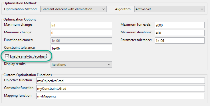
To enable gradients in the optimization algorithm, enable the Jacobian optimization option.
opt.OptimizationOptions.Jacobian = 'on';
To use analytic Jacobians when trimming models using Steady State Manager or the Model Linearizer, select the Enable analytic Jacobian trimming option.
Trim the model using the custom functions with gradients, and view the trimmed states.
[op4,rpt4] = findop(mdl,opspec,opt);
op4.States
ans =

x
__

(1.) scdTanks/Inertia
0
(2.) scdTanks/Tank1
15
(3.) scdTanks/Tank2
15
(4.) scdTanks/Tank3
16
The optimization result is the same as the result for the nongradient solution.
To see if the gradients improve the optimization efficiency, view the operating point search reports. For example, compare the number function evaluations for the solution:
Without gradients:
rpt3.OptimizationOutput.funcCount
ans =

    25
With gradients:
rpt4.OptimizationOutput.funcCount
ans =

     5
For this example, adding the analytical gradients decreases the number of function calls during optimization.
See Also
findop | operspec | getStateIndex | getInputIndex | getOutputIndex