Model Constant Propagation Delay

Open the model ConstantPropagationDelay. The model uses a Propagation Delay block to delay the output from a Sine Wave block by a constant value specified using a Constant block. The Sine Wave block is configured with a phase shift of pi/2, so the output is a cosine wave.

mdl = "ConstantPropagationDelay";
open_system(mdl)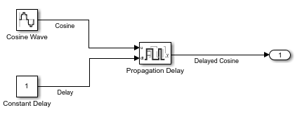

Simulate the model.

out = sim(mdl);

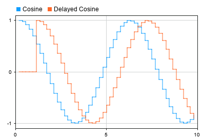
The Cosine and Delayed Cosine signals are plotted on the Dashboard Scope block. The Initial output value for the block is 0, so the value for the Delayed Cosine signal is 0 until the simulation time reaches 1 second. Then, the output becomes the first delayed Cosine value.

To understand how the Propagation Delay block affects the output signal sample time, display the sample time colors on the model and the timing legend. Then, update the block diagram.

1. On the Debug tab, under Diagnostics, click Information Overlays.

2. From the menu that appears, under Sample Time, select Colors and Timing Legend.

3. Press Ctrl+D to update the block diagram.

Alternatively, use the set_param function to enable the SampleTimeColors parameter for the model and to update the block diagram.

set_param(mdl,"SampleTimeColors","on")
set_param(mdl,"SimulationCommand","update")

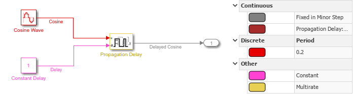
The sample time colors show that:

• The Cosine signal has a discrete sample rate of 0.2, defined by the Sine Wave block Sample time parameter.

• The Delay signal has constant sample time, defined by the Constant block Sample time parameter.

• The Propagation Delay block has multirate sample time.

• The Delayed Sine Wave signal has fixed-in-minor-step sample time.

The Timing Legend shows that the Propagation Delay block introduces an additional sample time, which is one of the rates for the multirate block. The additional variable sample time for the block allows the Propagation Delay block to update the output value as soon as the delay for a particular sample elapses in a variable-step simulation.

Now, run a fixed-step simulation using a different constant delay value and initial output value.

Configure the model to use a fixed-step solver.

1. On the Modeling tab, under Setup, click Model Settings.

2. In the Configuration Parameters dialog box, on the Solver tab, for the solver Type select Fixed-step.

3. In the Configuration Parameters dialog box, click OK.

Alternatively, use the set_param function to specify the SolverType parameter as Fixed-step.

set_param(mdl,"SolverType","Fixed-step")

When you use a fixed-step solver, you must configure the Propagation Delay block to run at a discrete rate.

1. Double-click the block to open the Block Parameters dialog box, or select the block and press Ctrl+Shift+I to display the Property Inspector.

2. Select Run at fixed time intervals.

3. Specify the Sample time as 0.1.

Alternatively, use the set_param function to configure the RunAtFixedTimeIntervals parameter and the SampleTime parameter.

set_param("ConstantPropagationDelay/Propagation Delay",...
    "RunAtFixedTimeIntervals","on","SampleTime","0.1")

For this simulation, in addition to using a fixed-step solver, specify a different value for the constant delay and initial output.

Specify the Initial output value for the Propagation Delay block as 0.5 using the Block Parameters dialog box, the Property Inspector, or the set_param function.

set_param("ConstantPropagationDelay/Propagation Delay",...
    "InitialOutput","0.5")

Configure the constant delay value as 0.5.

Specify the Value parameter for the Constant block as 0.5 using the Block Parameters dialog box, the Property Inspector, or the set_param function.

set_param("ConstantPropagationDelay/Constant Delay","Value","0.5")

Simulate the model again.

out = sim(mdl);

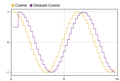
At the start of the simulation, the Delayed Sine signal value is 0.5. After the initial delay of 0.5 seconds, the output changes from the Initial output value to the delayed signal samples.

The sample time colors show that:

• The Cosine Wave signal has the discrete sample time of 0.2, defined by the Sine Wave Sample time parameter.

• The Delay signal has constant sample time, defined by the Constant block Sample time parameter.

• The Propagation Delay block has multirate sample time.

• The Delayed Sine Wave signal has discrete sample time.

The Timing Legend shows that the discrete sample time for the Delayed Sine Wave signal is 0.1, the same as the Sample time parameter value for the Propagation Delay block. The Propagation Delay block also introduces a controllable discrete rate with a minimum step size, or base rate, of 0.1.