Use Adaptive Zero-Crossing Location for More Robust Simulations

This example shows how the adaptive algorithm for zero-crossing location can improve simulation speed and robustness for systems that exhibit Zeno behavior, such as chattering.

When you enable zero-crossing detection, the software detects the occurrence of zero crossings and locates the time at which the zero crossing occurred through a process called bracketing. The Algorithm configuration parameter provides a choice of two zero-crossing location algorithms: Adaptive and Nonadaptive.

• The nonadaptive algorithm brackets every detected zero crossing until it locates the zero crossing. The algorithm defines the zero-crossing location as the time at which the zero-crossing signal value is within a small, fixed threshold near 0.

• The adaptive algorithm reduces the computational cost of locating zero crossings when systems exhibit Zeno behavior by:

  • Not bracketing detected zero crossings after the number of consecutive zero crossings exceeds the value specified by the Number of consecutive zero crossings parameter

  • Bracketing detected zero crossings only until the zero-crossing signal value is within the threshold of 0 specified by the Signal threshold parameter

Open Double Bouncing Ball Model

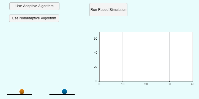
Open the model sldemo_doublebounce, which represents the dynamics of two balls that bounce on separate surfaces that change position at different times during simulation. A dashboard for the model opens along with the model.

mdl = "sldemo_doublebounce";
open_system(mdl)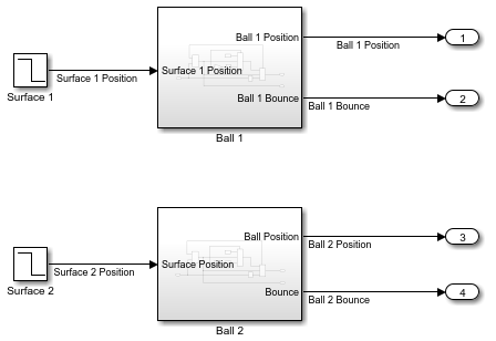

Each time a ball bounces, the ball changes direction, which means that the velocity of the ball changes sign and crosses zero. As the ball comes to rest, the system exhibits chattering as the height of each bounce and the time between bounces both decrease.

The dashboard for the model provides buttons to configure and run simulations and visualizes the motion of the balls and the surfaces on which they bounce. Simulations run by clicking Run Paced Simulation in the dashboard use simulation pacing to slow down the simulation so you can observe the animation of the bouncing balls.

Simulate Using Nonadaptive Zero-Crossing Location Algorithm

First, try to simulate the model using the nonadaptive algorithm. To observe the visualization of the system, use the dashboard to configure and run the simulation.

1. In the dashboard, click Use Nonadaptive Algorithm.

2. Click Run Paced Simulation.

Alternatively, create a Simulink.SimulationInput object to configure the simulation. Then, run the simulation programmatically using the sim function. Enable the CaptureErrors parameter on the SimulationInput object to ensure that the sim function returns simulation results even if the software issues an error during the simulation.

simin = Simulink.SimulationInput(mdl);
simin = setModelParameter(simin,CaptureErrors="on");
simin = setModelParameter(simin,ZeroCrossAlgorithm="Nonadaptive");

out = sim(simin);

The software issues an error because the number of consecutive zero crossings exceeds the specified limit due to the chattering that occurs as the ball comes to rest.

err = out.ErrorMessage

err = 
    'Simulink will stop the simulation of model 'sldemo_doublebounce' because the 1 zero crossing signal(s) identified below caused 1000 consecutive zero crossing events in time interval between 15.290515947658548 and 15.290568558574787.
      --------------------------------------------------------------------------------
     Number of consecutive zero-crossings : 1000
                Zero-crossing signal name : RelopInput
                               Block type : RelationalOperator
                               Block path : 'sldemo_doublebounce/Ball 1/Detect Bounce'
     --------------------------------------------------------------------------------
      
     Suggested Actions:
         •  You can suppress the diagnostics and continue simulation without bracketing these zero crossings by switching the  zero crossing detection algorithm to 'Adaptive' and setting the Ignored Zero Crossings diagnostic to 'none'. - Fix
         •  Disable zero-crossing detection on the blocks listed above that caused the most events.
     '

To analyze the simulation results, plot the positions of Ball 1 and Ball 2.

y = out.yout;
b1 = getElement(y,"Ball 1 Position");
b2 = getElement(y,"Ball 2 Position");

figure
plot(b1.Values)
hold on
plot(b2.Values)
title("Nonadaptive Zero-Crossing Location Simulation Results")
legend("Ball 1","Ball 2")
ylim([0 70])
xlim([0 42])

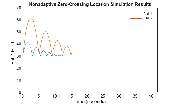
The simulation stops after about 15 seconds, as the velocity of Ball 1 approaches zero. The number of consecutive zero crossings exceeds the limit before either surface changes position. Using the nonadaptive algorithm, the simulation cannot proceed to provide information about how the system responds to the position changes.

Simulate Using Adaptive Zero-Crossing Location Algorithm

To see the difference between the nonadaptive and adaptive zero-crossing location algorithms, simulate the model again using the adaptive algorithm. To observe the visualization of the system, use the dashboard to configure and run the simulation.

1. In the dashboard, click Use Adaptive Algorithm.

2. Click Run Paced Simulation.

Alternatively, configure and run the simulation using a Simulink.SimulationInput object and the sim function.

simin = setModelParameter(simin,ZeroCrossAlgorithm="Adaptive");

out = sim(simin);

Warning: At time 15.177695754911614 and step size of 0.024288703254423893, found 1 zero crossing(s) due to the signal(s) listed below. However, the adaptive zero-crossing detection algorithm is not reducing the step size any further because the magnitude of the signal(s) with zero crossing(s) is less than tolerance (0.001) during this time step.
 --------------------------------------------------------------------------------
          Zero-crossing signal index : 1
           Zero-crossing signal name : RelopInput
                          Block type : RelationalOperator
                          Block path : '<a href="matlab:open_and_hilite_hyperlink ('sldemo_doublebounce/Ball 1/Detect Bounce','error')">sldemo_doublebounce/Ball 1/Detect Bounce</a>'
--------------------------------------------------------------------------------
 
Suggested Actions:
    •  Turn off this diagnostic by setting 'Ignored Zero Crossings' to 'none'. - <a href="matlab:set_param('sldemo_doublebounce','IgnoredZcDiagnostic','none');">Fix</a>
    •  Disabling zero-crossing detection on the blocks listed above can speed up simulation.

The simulation completes, and the software issues a warning when the adaptive zero-crossing location algorithm does not bracket a detected zero crossing.

The adaptive algorithm can improve simulation performance and robustness but can also reduce accuracy in some cases by ignoring detected zero crossings. By default, the software issues a warning when the adaptive algorithm ignores zero crossings. To suppress these warnings, set the Ignored zero crossings configuration parameter to None.

1. Open the Configuration Parameters dialog box. On the Modeling tab, click Model Settings.

2. In the Configuration Parameters dialog box, on the Diagnostics pane, expand Advanced parameters.

3. From the Ignored zero crossings list, select none.

4. Click OK.

To analyze the simulation results, plot the positions of Ball 1 and Ball 2.

y = out.yout;
b1 = getElement(y,"Ball 1 Position");
b2 = getElement(y,"Ball 2 Position");

figure
plot(b1.Values)
hold on
plot(b2.Values)
title("Adaptive Zero-Crossing Location Simulation Results")
legend("Ball 1","Ball 2")
ylim([0 70])
xlim([0 42])

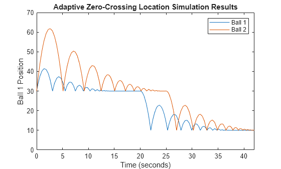
At the start of the simulation, each ball starts from the same position, in contact with the surface, and with a different initial velocity.

• The velocity of Ball 1 approaches zero after about 10 seconds. Ball 1 is approximately at rest until about 20 seconds, when the first surface drops.

• The velocity of Ball 2 approaches zero after about 20 seconds. Ball 2 is approximately at rest until about 25 seconds, when the second surface drops.

Explore Zero-Crossing Location Algorithms Further

To demonstrate the difference between the adaptive and nonadaptive zero-crossing location algorithms, this example sets the value of the Time tolerance model configuration parameter to 1e-7. The Time tolerance parameter defines the time interval in which detected zero crossings are considered consecutive. This example uses a larger time tolerance to ensure that simulations run using the nonadaptive algorithm issue an error about too many consecutive zero crossings instead of slowing down significantly.

To explore the zero-crossing location algorithms further, try running simulations with the adaptive and nonadaptive algorithms using the default value of the Time tolerance. parameter. To change the value of the Time tolerance parameter, use the Configuration Parameters dialog box.

1. On the Modeling tab, under Setup, click Model Settings.

2. In the Configuration Parameters dialog box, select the Solver pane and expand Solver details.

3. In the Zero-crossing options section, in the Time tolerance box, enter 10*128*eps.

4. Click OK.

When you use the nonadaptive algorithm with the default Time tolerance value, the simulation slows down significantly due to the chattering that happens as the velocity of the first ball approaches 0.