Perform Global Sensitivity Analysis by Computing First- and Total-Order Sobol Indices

Load the tumor growth model.

sbioloadproject tumor_growth_vpop_sa.sbproj

Get a variant with the estimated parameters and the dose to apply to the model.

v = getvariant(m1);
d = getdose(m1,'interval_dose');

Get the active configset and set the tumor weight as the response.

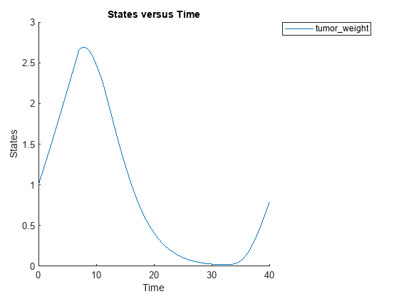
cs = getconfigset(m1);
cs.RuntimeOptions.StatesToLog = 'tumor_weight';

Simulate the model and plot the tumor growth profile.

sbioplot(sbiosimulate(m1,cs,v,d));

Perform global sensitivity analysis (GSA) on the model to find the model parameters that the tumor growth is sensitive to.

First, retrieve model parameters of interest that are involved in the pharmacodynamics of the tumor growth. Define the model response as the tumor weight.

modelParamNames = {'L0','L1','w0','k1','k2'};
outputName = 'tumor_weight';

Then perform GSA by computing the first- and total-order Sobol indices using sbiosobol. Set 'ShowWaitBar' to true to show the simulation progress. By default, the function uses 1000 parameter samples to compute the Sobol indices [1].

rng('default');
sobolResults = sbiosobol(m1,modelParamNames,outputName,Variants=v,Doses=d,ShowWaitBar=true)

sobolResults = 
  Sobol with properties:

                Time: [444x1 double]
        SobolIndices: [5x1 struct]
            Variance: [444x1 table]
    ParameterSamples: [1000x5 table]
         Observables: {'[Tumor Growth].tumor_weight'}
      SimulationInfo: [1x1 struct]

You can change the number of samples by specifying the 'NumberSamples' name-value pair argument. The function requires a total of (number of input parameters + 2) * NumberSamples model simulations.

Show the mean model response, the simulation results, and a shaded region covering 90% of the simulation results.

plotData(sobolResults,ShowMedian=true,ShowMean=false);

You can adjust the quantile region to a different percentage by specifying 'Alphas' for the lower and upper quantiles of all model responses. For instance, an alpha value of 0.1 plots a shaded region between the 100 * alpha and 100 * (1 - alpha) quantiles of all simulated model responses.

plotData(sobolResults,Alphas=0.1,ShowMedian=true,ShowMean=false);

Plot the time course of the first- and total-order Sobol indices.

h = plot(sobolResults);
% Resize the figure.
h.Position(:) = [100 100 1280 800];

The first-order Sobol index of an input parameter gives the fraction of the overall response variance that can be attributed to variations in the input parameter alone. The total-order index gives the fraction of the overall response variance that can be attributed to any joint parameter variations that include variations of the input parameter.

From the Sobol indices plots, parameters L1 and w0 seem to be the most sensitive parameters to the tumor weight before the dose was applied at t = 7. But after the dose is applied, k1 and k2 become more sensitive parameters and contribute most to the after-dosing stage of the tumor weight. The total variance plot also shows a larger variance for the after-dose stage at t > 35 than for the before-dose stage of the tumor growth, indicating that k1 and k2 might be more important parameters to investigate further. The fraction of unexplained variance shows some variance at around t = 33, but the total variance plot shows little variance at t = 33, meaning the unexplained variance could be insignificant. The fraction of unexplained variance is calculated as 1 - (sum of all the first-order Sobol indices), and the total variance is calculated using var(response), where response is the model response at every time point.

You can also display the magnitudes of the sensitivities in a bar plot. Darker colors mean that those values occur more often over the whole time course.

bar(sobolResults);

You can specify more samples to increase the accuracy of the Sobol indices, but the simulation can take longer to finish. Use addsamples to add more samples. For example, if you specify 1500 samples, the function performs 1500 * (2 + number of input parameters) simulations.

gsaMoreSamples = addsamples(gsaResults,1500)

The SimulationInfo property of the result object contains various information for computing the Sobol indices. For instance, the model simulation data (SimData) for each simulation using a set of parameter samples is stored in the SimData field of the property. This field is an array of SimData objects.

sobolResults.SimulationInfo.SimData

 
   SimBiology SimData Array : 1000-by-7
 
   Index:    Name:         ModelName:         DataCount: 
   1           -           Tumor Growth Model 1          
   2           -           Tumor Growth Model 1          
   3           -           Tumor Growth Model 1          
   ...                                                   
   7000        -           Tumor Growth Model 1          
 

You can find out if any model simulation failed during the computation by checking the ValidSample field of SimulationInfo. In this example, the field shows no failed simulation runs.

all(sobolResults.SimulationInfo.ValidSample)

ans = 1x7 logical array

   1   1   1   1   1   1   1

SimulationInfo.ValidSample is a table of logical values. It has the same size as SimulationInfo.SimData. If ValidSample indicates that any simulations failed, you can get more information about those simulation runs and the samples used for those runs by extracting information from the corresponding column of SimulationInfo.SimData. Suppose that the fourth column contains one or more failed simulation runs. Get the simulation data and sample values used for that simulation using getSimulationResults.

[samplesUsed,sd,validruns] = getSimulationResults(sobolResults,4);

You can add custom expressions as observables and compute Sobol indices for the added observables. For example, you can compute the Sobol indices for the maximum tumor weight by defining a custom expression as follows.

% Suppress an information warning that is issued during simulation.
warnSettings = warning('off', 'SimBiology:sbservices:SB_DIMANALYSISNOTDONE_MATLABFCN_UCON');
% Add the observable expression.
sobolObs = addobservable(sobolResults,'Maximum tumor_weight','max(tumor_weight)','Units','gram');

Plot the computed simulation results showing the 90% quantile region.

h2 = plotData(sobolObs,ShowMedian=true,ShowMean=false);
h2.Position(:) = [100 100 1280 800];

You can also remove the observable by specifying its name.

gsaNoObs = removeobservable(sobolObs,'Maximum tumor_weight');

Restore the warning settings.

warning(warnSettings);