Nonlinear Regression
What is Nonlinear Regression?
The purpose of regression models is to describe a response variable as a function of independent variables. Multiple linear regression models describe the response as a linear combination of coefficients and functions of independent variables. Nonlinearities can be modeled using nonlinear functions of independent variables. However, the coefficients always enter the model in a linear fashion.
Nonlinear regression models are more mechanistic models of nonlinear relationships between the response and independent variables. The parameters can enter the model as exponential, trigonometric, power, or any other nonlinear function. The unknown parameters in the model are estimated by minimizing a statistical criterion such as the negative log likelihood or the sum of squared deviations between observed and predicted values.
In the case of pharmacokinetic (PK) studies, the response data usually represent some measured drug concentrations, and independent variables are often dose and time. The nonlinear function often used for such data is an exponential function since many drugs once distributed in a patient are eliminated in an exponential fashion. One PK parameter to estimate in this case is the rate at which the drug is eliminated from the body given the concentration-time data.
For instance, consider drug plasma concentration data from a single individual after an intravenous bolus dose measured at different time points with some errors. Assume the measured drug concentration follows a monoexponential decline: .
This model describes the time course of drug concentration in the body (Ct), as a function of the drug concentration after an intravenous bolus dose at t = 0 (C0), time (t), and elimination rate parameter (ke). ε is the mean-zero and unit-variance variable, that is, representing the measurement error and a is the error model parameter (here, standard deviation).
More generically, you can write the model as
where yi is the ith response (such as drug concentration), f is a function of time t and model parameters p (such as ke), and an error model .
Fitting Options in SimBiology
This table summarizes nonlinear regression options available in SimBiology®.
| Fitting Option | Example |
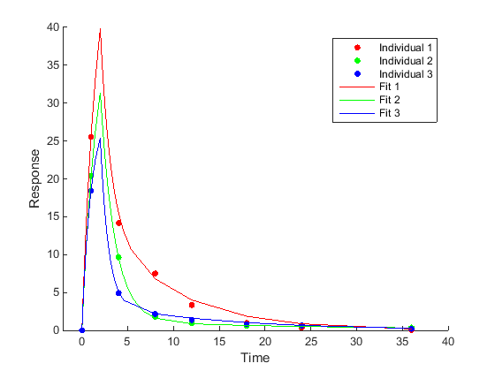
Individual-specific parameter estimation (Unpooled fitting) Fit each individual separately, resulting in one set of parameter estimates for each individual. |
|
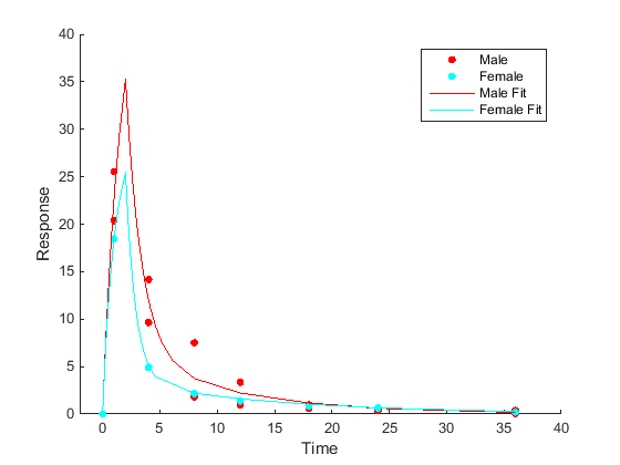
Category- or group-specific parameter estimation Fit each category or group separately, resulting in one set of parameter estimates for each category. |
|
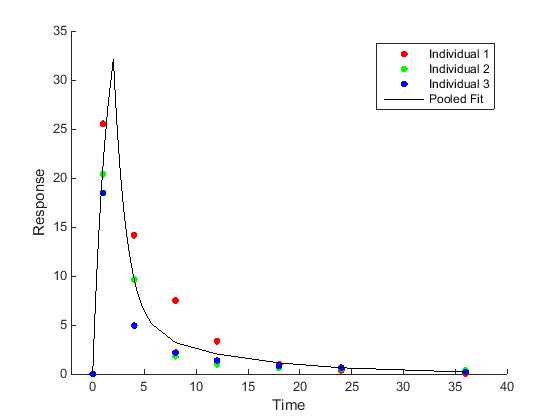
Population-wide parameter estimation (Pooled fitting) Fit all of the data pooled together, resulting in just one set of parameter estimates. |
|
In addition, SimBiology supports four kinds of error models for measured or observed responses, namely, constant (default), proportional, combined, and exponential. For details, see Error Models. Depending on the optimization method, you can specify an error model for each response or all responses. For details, see Supported Methods for Parameter Estimation in SimBiology.
Parameter Transformations
SimBiology supports three parameter transformations. These parameter transformations can be useful to improve fitting convergence or to enforce parameter bounds.
The general model explained previously is , where p is model parameters that you can transform. Consider the following two equations.
Here, represents transformed model parameters,
p represents untransformed model
parameters, T is the transformation, and
T-1 is the
inverse transformation.
SimBiology performs parameter estimation using the transformed parameters
β, which means that the transformed model is used, where F is the model function using
the transformed parameters. Equivalently, the model function can be rewritten as .
In other words, the SimBiology optimizer uses the transformed values during maximum likelihood estimation but the reported fit result is reverted back to the model space (untransformed values). For example, if you are estimating a clearance parameter Cl that is log-transformed, you have Clβ = log(Cl), where Clβ is what the optimizer uses and Cl is what the model sees.
Specifying parameter transformations imposes implicit bounds on the untransformed
parameter values. The log transformation keeps the parameter
value to be always positive, and the logit and
probit transformations keep the parameter value to between
0 and 1. Alternatively, you can specify
further constraints on the parameter values by providing explicit bounds for
untransformed parameters p or for the transformed parameters
β.
| Transformation | Transformed Parameter and Range† | Untransformed Parameter and Range‡ | Description |
|---|---|---|---|
| In many cases, the Applying the | ||
logit | The | ||
probit | Similar to |
† Use the InitialTransformedValue and
TransformedBounds properties of an EstimatedInfo object to set the
initial transformed value and transformed bounds to the desired subset of the
range.
‡ Use the InitialValue and Bounds
properties of an EstimatedInfo object to set the
initial untransformed value and untransformed bounds to the desired subset of the
range.
Maximum Likelihood Estimation
SimBiology estimates parameters by the method of maximum likelihood. Rather than directly
maximizing the likelihood function, SimBiology constructs an equivalent minimization problem. Whenever possible, the estimation
is formulated as a weighted least squares (WLS) optimization
that minimizes the sum of the squares of weighted residuals. Otherwise, the estimation is
formulated as the minimization of the negative of the logarithm of the likelihood (NLL). The WLS formulation often
converges better than the NLL formulation, and SimBiology can take advantage of specialized WLS algorithms,
such as the Levenberg-Marquardt algorithm implemented in lsqnonlin and
lsqcurvefit. SimBiology uses WLS when there is a single error model that
is constant, proportional, or exponential. SimBiology uses NLL if you have a combined error model or a
multiple-error model, that is, a model having an error model for each response.
sbiofit supports different
optimization methods, and passes in the formulated WLS or
NLL expression to the optimization method that minimizes
it. For simplicity, each expression shown below assumes only one error model and one response.
If there are multiple responses, SimBiology takes the sum of the expressions that correspond to error models of given
responses.
| Expression that is being minimized | |
|---|---|
| Weighted Least Squares (WLS) | For the constant error model, |
| For the proportional error model, | |
| For the exponential error model, | |
| For numeric weights, | |
| Negative Log-likelihood (NLL) | For the combined error model and multiple-error model, |
The variables are defined as follows.
N | Number of experimental observations |
yi | The ith experimental observation |
Predicted value of the ith observation | |
Standard deviation of the ith observation.
| |
The weight of the ith predicted value | |
When you use numeric weights or the weight function, the weights are assumed to be inversely proportional to the variance of the error, that is, where a is the constant error parameter. If you use weights, you cannot specify an error model except the constant error model.
Various optimization methods have different requirements on the function that is being minimized. For some methods, the estimation of model parameters is performed independently of the estimation of the error model parameters. The following table summarizes the error models and any separate formulas used for the estimation of error model parameters, where a and b are error model parameters and e is the standard mean-zero and unit-variance (Gaussian) variable.
| Error Model | Error Parameter Estimation Function |
|---|---|
'constant': | |
'exponential': | |
'proportional': | |
'combined': | Error parameters are included in the minimization. |
| Weights |
Note
nlinfit only support single error models, not multiple-error models, that is, response-specific error models. For a combined error model, it uses an iterative WLS algorithm. For other error models, it uses the WLS algorithm as described previously. For details, see nlinfit (Statistics and Machine Learning Toolbox).
Fitting Workflow
The following steps show one of the workflows you can use at the command line to fit a PK model.
Convert the data to the
groupedDataformat.Define dosing data. For details, see Doses in SimBiology Models.
Create a structural model (one-, two-, or a multicompartment model). For details, see Create Pharmacokinetic Models.
Map the response variable from data to the model component. For example, if you have the measured drug concentration data for the central compartment, then map it to the drug species in the central compartment (typically the
Drug_Centralspecies).Specify parameters to estimate using an
EstimatedInfo object. Optionally, you can specify parameter transformations, initial values, and parameter bounds.Perform parameter estimation using
sbiofitorfitproblem.
For illustrated examples, see the following.
See Also
sbiofit | groupedData | estimatedInfo | sbiofitmixed