Fit Two-Compartment Model to PK Profiles of Multiple Individuals
Estimate pharmacokinetic parameters of multiple individuals using a two-compartment model.
Suppose you have drug plasma concentration data from three individuals that you want
to use to estimate corresponding pharmacokinetic parameters, namely the volume of
central and peripheral compartment (Central,
Peripheral), the clearance rate (Cl_Central),
and intercompartmental clearance (Q12). Assume the drug concentration
versus the time profile follows the biexponential decline , where Ct is the drug
concentration at time t, and a and
b are slopes for corresponding exponential declines.
The synthetic data set contains drug plasma concentration data measured in both central and peripheral compartments. The data was generated using a two-compartment model with an infusion dose and first-order elimination. These parameters were used for each individual.
Central | Peripheral | Q12 | Cl_Central | |
|---|---|---|---|---|
| Individual 1 | 1.90 | 0.68 | 0.24 | 0.57 |
| Individual 2 | 2.10 | 6.05 | 0.36 | 0.95 |
| Individual 3 | 1.70 | 4.21 | 0.46 | 0.95 |
The data is stored as a table with variables ID, Time, CentralConc, and PeripheralConc. It represents the time course of plasma concentrations measured at eight different time points for both central and peripheral compartments after an infusion dose.
load('data10_32R.mat')
Convert the data set to a groupedData object which is the required
data format for the fitting function sbiofit for later use. A
groupedData object also lets you set independent variable and
group variable names (if they exist). Set the units of the ID,
Time, CentralConc, and
PeripheralConc variables. The units are optional and only
required for the UnitConversion feature, which
automatically converts matching physical quantities to one consistent unit
system.
gData = groupedData(data);
gData.Properties.VariableUnits = {'','hour','milligram/liter','milligram/liter'};
gData.Properties
ans =

  struct with fields:

                Description: ''
                   UserData: []
             DimensionNames: {'Row'  'Variables'}
              VariableNames: {'ID'  'Time'  'CentralConc'  'PeripheralConc'}
              VariableTypes: ["double"    "double"    "double"    "double"]
       VariableDescriptions: {}
              VariableUnits: {''  'hour'  'milligram/liter'  'milligram/liter'}
         VariableContinuity: []
                   RowNames: {}
           CustomProperties: [1×1 matlab.tabular.CustomProperties]
          GroupVariableName: 'ID'
    IndependentVariableName: 'Time'
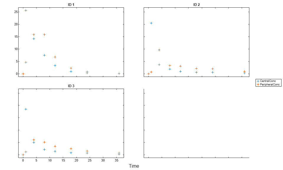
Create a trellis plot that shows the PK profiles of three individuals.
sbiotrellis(gData,'ID','Time',{'CentralConc','PeripheralConc'},...
            'Marker','+','LineStyle','none');
Use the built-in PK library to construct a two-compartment model with infusion dosing and first-order elimination where the elimination rate depends on the clearance and volume of the central compartment. Use the configset object to turn on unit conversion.
pkmd                 = PKModelDesign;
pkc1                 = addCompartment(pkmd,'Central');
pkc1.DosingType      = 'Infusion';
pkc1.EliminationType = 'linear-clearance';
pkc1.HasResponseVariable = true;
pkc2                 = addCompartment(pkmd,'Peripheral');
model                = construct(pkmd);
configset            = getconfigset(model);
configset.CompileOptions.UnitConversion = true;
Assume every individual receives an infusion dose at time = 0, with a total infusion amount of 100 mg at a rate of 50 mg/hour. For details on setting up different dosing strategies, see Doses in SimBiology Models.
dose             = sbiodose('dose','TargetName','Drug_Central');
dose.StartTime   = 0;
dose.Amount      = 100;
dose.Rate        = 50;
dose.AmountUnits = 'milligram';
dose.TimeUnits   = 'hour';
dose.RateUnits   = 'milligram/hour';
The data contains measured plasma concentrations in the central and peripheral compartments. Map these variables to the appropriate model species, which are Drug_Central and Drug_Peripheral.
responseMap = {'Drug_Central = CentralConc','Drug_Peripheral = PeripheralConc'};
The parameters to estimate in this model are the volumes of central and peripheral compartments (Central and Peripheral), intercompartmental clearance Q12, and clearance rate Cl_Central. In this case, specify log-transform for Central and Peripheral since they are constrained to be positive. The estimatedInfo object lets you specify parameter transforms, initial values, and parameter bounds (optional).
paramsToEstimate   = {'log(Central)','log(Peripheral)','Q12','Cl_Central'};
estimatedParam     = estimatedInfo(paramsToEstimate,'InitialValue',[1 1 1 1]);
Fit the model to all of the data pooled together, that is, estimate one set of parameters for all individuals. The default estimation method that sbiofit uses will change depending on which toolboxes are available. To see which estimation function sbiofit used for the fitting, check the EstimationFunction property of the corresponding results object.
pooledFit = sbiofit(model,gData,responseMap,estimatedParam,dose,'Pooled',true)
pooledFit =

  OptimResults with properties:

                   ExitFlag: 3
                     Output: [1×1 struct]
                  GroupName: []
                       Beta: [4×3 table]
         ParameterEstimates: [4×3 table]
                          J: [24×4×2 double]
                       COVB: [4×4 double]
           CovarianceMatrix: [4×4 double]
                          R: [24×2 double]
                        MSE: 6.6220
                        SSE: 291.3688
                    Weights: []
              LogLikelihood: -111.3904
                        AIC: 230.7808
                        BIC: 238.2656
                        DFE: 44
             DependentFiles: {1×3 cell}
                       Data: [24×4 groupedData]
    EstimatedParameterNames: {'Central'  'Peripheral'  'Q12'  'Cl_Central'}
             ErrorModelInfo: [1×3 table]
         EstimationFunction: 'lsqnonlin'
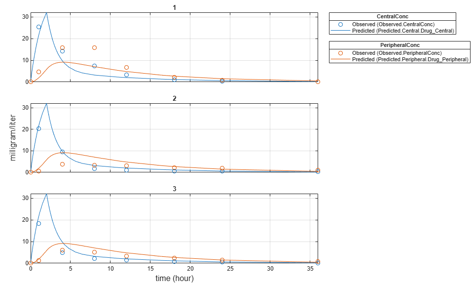
Plot the fitted results versus the original data. Although three separate plots were generated, the data was fitted using the same set of parameters (that is, all three individuals had the same fitted line).
plot(pooledFit);
Estimate one set of parameters for each individual and see if there is any improvement in the parameter estimates. In this example, since there are three individuals, three sets of parameters are estimated.
unpooledFit = sbiofit(model,gData,responseMap,estimatedParam,dose,'Pooled',false);
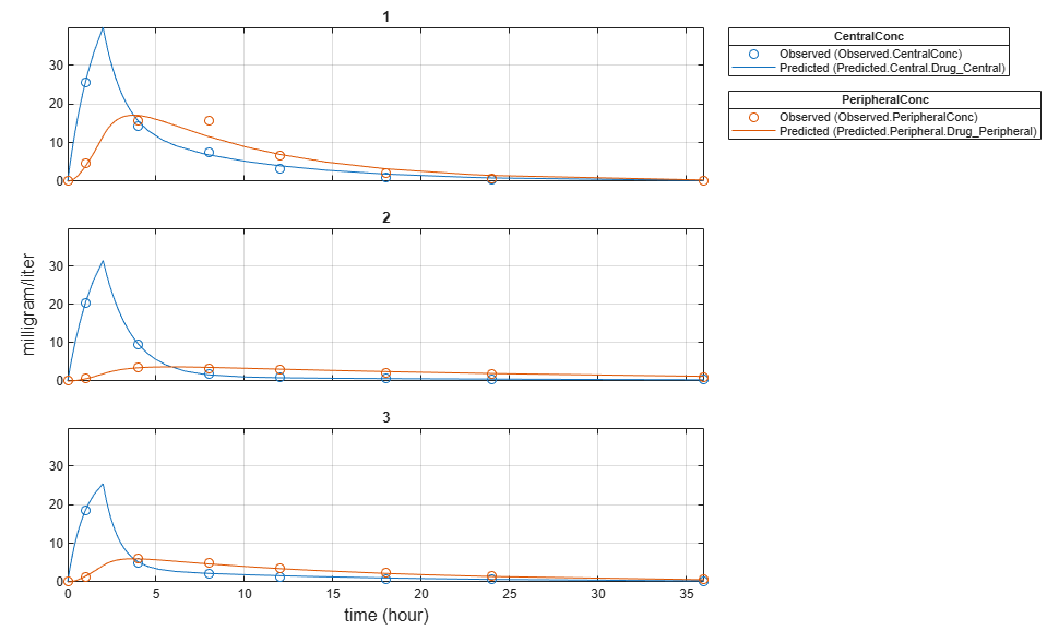
Plot the fitted results versus the original data. Each individual was fitted differently (that is, each fitted line is unique to each individual) and each line appeared to fit well to individual data.
plot(unpooledFit);
Display the fitted results of the first individual. The MSE was lower than that of the pooled fit. This is also true for the other two individuals.
unpooledFit(1)
ans =

  OptimResults with properties:

                   ExitFlag: 3
                     Output: [1×1 struct]
                  GroupName: 1
                       Beta: [4×3 table]
         ParameterEstimates: [4×3 table]
                          J: [8×4×2 double]
                       COVB: [4×4 double]
           CovarianceMatrix: [4×4 double]
                          R: [8×2 double]
                        MSE: 2.1380
                        SSE: 25.6559
                    Weights: []
              LogLikelihood: -26.4805
                        AIC: 60.9610
                        BIC: 64.0514
                        DFE: 12
             DependentFiles: {1×3 cell}
                       Data: [8×4 groupedData]
    EstimatedParameterNames: {'Central'  'Peripheral'  'Q12'  'Cl_Central'}
             ErrorModelInfo: [1×3 table]
         EstimationFunction: 'lsqnonlin'
Generate a plot of the residuals over time to compare the pooled and unpooled fit results. The figure indicates unpooled fit residuals are smaller than those of pooled fit as expected. In addition to comparing residuals, other rigorous criteria can be used to compare the fitted results.
t = [gData.Time;gData.Time];
res_pooled = vertcat(pooledFit.R);
res_pooled = res_pooled(:);
res_unpooled = vertcat(unpooledFit.R);
res_unpooled = res_unpooled(:);
plot(t,res_pooled,'o','MarkerFaceColor','w','markerEdgeColor','b')
hold on
plot(t,res_unpooled,'o','MarkerFaceColor','b','markerEdgeColor','b')
refl = refline(0,0); % A reference line representing a zero residual
title('Residuals versus Time');
xlabel('Time');
ylabel('Residuals');
legend({'Pooled','Unpooled'});

This example showed how to perform pooled and unpooled estimations using sbiofit. As illustrated, the unpooled fit accounts for variations due to the specific subjects in the study, and, in this case, the model fits better to the data. However, the pooled fit returns population-wide parameters. If you want to estimate population-wide parameters while considering individual variations, use sbiofitmixed.