Design and Analyze Microstrip-to-Stripline Transition for Multilayer Printed Circuit Board

This example shows how to design and analyze a microstrip-to-stripline (MS-to-SL) vertical transition for multilayer printed circuit boards (PCBs), which is essential for high-speed digital and RF applications.

Create Variables

The image below shows a top view of a multilayer PCB featuring a transition from a grounded coplanar waveguide (GCPW) to a stripline. The colors yellow, blue, and red represent the metal on the first, second, and third layers, respectively.The second metal layer acts as a ground plane of GCPW. The third metal layer is a stripline with equal distance from top GCPW and the ground plane at the very bottom of a mlutiplayer PCB.

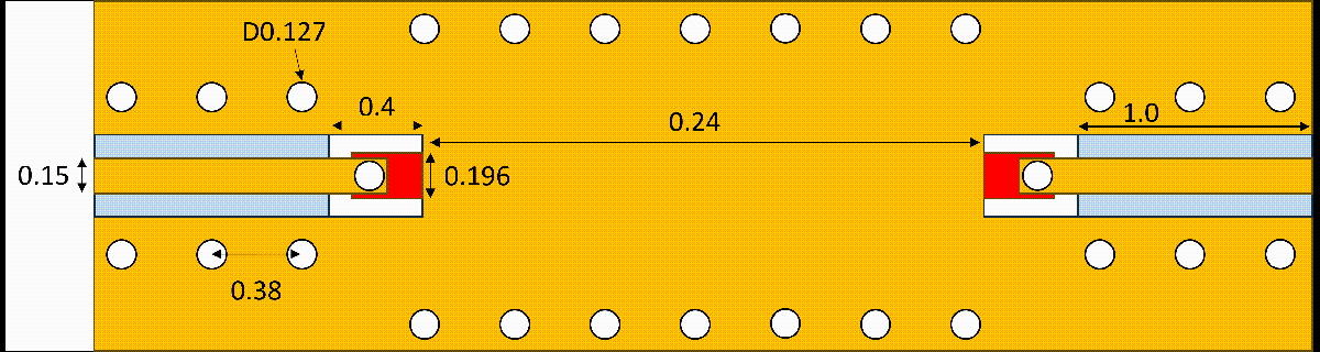
Create variables for the MS-to-SL transition.

wBoard = 1.5e-3; % Board width
lBoard = 5.2e-3; % Board length
wCPW = 0.15e-3; % Width of coplanar trace
lCPW = 1.25e-3; % Length of coplanar trace
sCPW = 0.1e-3; % Space between coplanar trace and ground
lTrans = 0.4e-3; % Length of transition area
lGCPW = 1e-3; % Length of grounded coplanar waveguide in second layer
wSline = 0.196e-3; % Width of stripline
lSline = 3e-3; % Length of stripline
dVia = 0.127e-3; % Via diameter
sxVia = 0.381e-3; % Space between GRVs in x-direction.
epsR = 5.9; % Dielectric constant of substrate
tSub = 96.5e-6; % Substrate thickness

Create Microstrip-to-Stripline Transition

Use the antenna.Rectangle to create a shape of the PC board.

board = antenna.Rectangle(Width=wBoard,Length=lBoard);

Create a signal trace of the GCPW in the top layer.

lineCPW = antenna.Rectangle(Width=wCPW,Length=lCPW);
lineCPW = translate(lineCPW,[-0.5*(lBoard-lCPW) 0 0]);
lineCPW = lineCPW+mirrorY(copy(lineCPW));

Create a ground plane of the GCPW in the top layer.

gndCPW1 = copy(board);
rect = antenna.Rectangle(Width=wCPW+2*sCPW,Length=lTrans+lGCPW);
rect = translate(rect,[-0.5*(lBoard-rect.Length) 0 0]);
rect = rect+mirrorY(copy(rect));
gndCPW1 = gndCPW1-rect;

Unite a signal trace and ground plane of the GCPW in the top layer using + function.

mGCPW = lineCPW+gndCPW1;

Visualize the top layer of a PCB.

figure
show(mGCPW)

Create a ground plane of the GCPW in the second layer.

gndCPW2 = antenna.Rectangle(Width=wBoard,Length=lGCPW);
gndCPW2 = translate(gndCPW2,[-0.5*(lBoard-lGCPW) 0 0]);
gndCPW2 = gndCPW2+mirrorY(copy(gndCPW2));

Use antenna.Rectangle to create a stripline trace in the third layer.

lineSL = antenna.Rectangle(Width=wSline,Length=lSline);

Use the dielectric object to create a substrate.

sub1 = dielectric(EpsilonR=epsR,Thickness=tSub);
sub2 = dielectric(EpsilonR=epsR,Thickness=2*tSub);
sub3 = dielectric(EpsilonR=epsR,Thickness=3*tSub);

Use the pcbComponent object to create a multilayer PCB.

p = pcbComponent( ...
    BoardShape = board, ...
    BoardThickness = 6*tSub, ...
    Layers = {mGCPW sub1 gndCPW2 sub2 lineSL sub3 board}, ...
    FeedDiameter = wCPW, ...
    ViaDiameter = dVia, ...
    FeedViaModel = 'hexagon');

Set the feeds at the both ends of GCPW signal trace.

p.FeedLocations = [
    -0.5*lBoard 0 1 3
    0.5*lBoard 0 1 3];

Set the two transition vias between the GCPW and the SL, and twenty six ground return vias (GRVs) between the GCPW and the bottommost ground plane.

xv1 = sxVia*(-1:1:1)';
yv1 = 0.275e-3;
xv2 = sxVia*(-3:1:3)';
yv2 = 0.5*wBoard-dVia;
p.ViaLocations = [
     1.425e-3 0 1 5
    -1.425e-3 0 1 5
    xv1-0.5*lBoard+0.5e-3 [yv1 1 7].*ones(size(xv1))
    xv1-0.5*lBoard+0.5e-3 [-yv1 1 7].*ones(size(xv1))
    xv1+0.5*lBoard-0.5e-3 [yv1 1 7].*ones(size(xv1))
    xv1+0.5*lBoard-0.5e-3 [-yv1 1 7].*ones(size(xv1))
    xv2 [yv2 1 7].*ones(size(xv2))
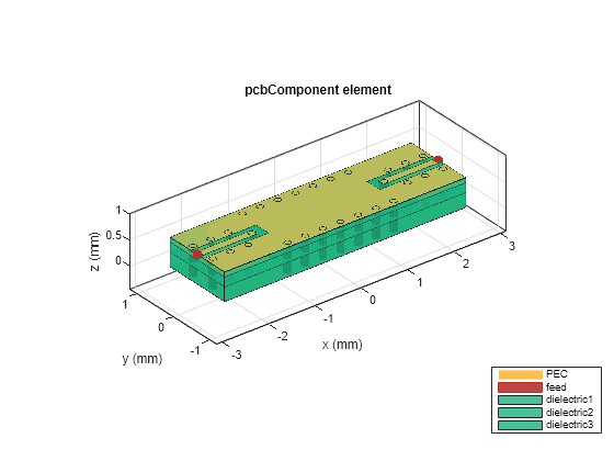
    xv2 [-yv2 1 7].*ones(size(xv2))];

Visualize the multilayer PCB with the MS-to-SL transition

figure
show(p)

Use the mesh function to mesh the multilayer PCB.

warning('off','MATLAB:polyshape:repairedBySimplify')
figure
mesh(p,MaxEdgeLength=5e-4)

warning('on','MATLAB:polyshape:repairedBySimplify')

Analyze Microstrip-to-Stripline Transition

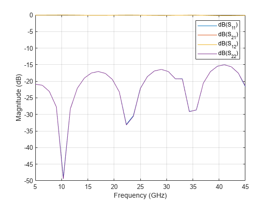
Use the sparameters function to calculate the S-parameters.

freq = linspace(5e9,45e9,31);
s = sparameters(p,freq);

Plot the S-parameters.

figure
rfplot(s)