Design, Visualize and Explore Inverse Chebyshev Filter - II
This example shows how to design a fourth-order inverse Chebyshev low-pass filter with stopband frequency of 10000 rad/sec, and epsilon of 0.01 (please see the reference section) using rffilter. This rffilter could be used in a circuit or in a rfbudget object.
The rffilter object is used to design a RF filter. A filter requires a minimum set for parameters to completely define it.
The parameters to design an inverse Chebyshev filter can be one of the following:
Filter order, Passband frequency, Passband and Stopband Attenuation
Passband and Stopband frequencies, Passband and Stopband Attenuation
Filter order, Stopband frequency, Stopband Attenuation
Design Filter
N           = 4;                                    % Filter order
Fs          = 1000/(2*pi);                          % Stopband frequency
epsilon     = 0.01;
Rs          = 10*log10((1+epsilon^2)/epsilon^2);    % Stopband attenuation
Use the first set of parameters to define the filter.
r = rffilter(FilterType="InverseChebyshev",ResponseType="Lowpass",  ...
    Implementation="Transfer function",FilterOrder=N,               ...
    PassbandFrequency=Fs,PassbandAttenuation=Rs,                    ...
    StopbandAttenuation=Rs);
Note: Alternative, you can also use the third set of parameters to design the same filter:
r = rffilter(FilterType="InverseChebyshev",ResponseType="Lowpass",  ...
Implementation="Transfer function",FilterOrder=N,                   ...
StopbandFrequency=Fs,StopbandAttenuation=Rs);
The limitation of this parameter set is that it assumes the passband attenuation to be fixed at 10*log10(2) dB.
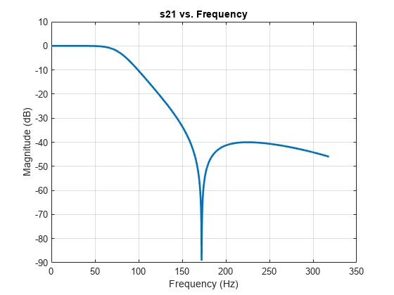
Visualize Magnitude Response, Phase Response, and Phase Delay of Filter
frequencies = linspace(0,2*Fs,1001);
rfplot(r, frequencies);


Optionally, you can also use Signal Processing Toolbox™ to visualize the analog filter using:
freqs(numerator{2,1},denominator)
Find Zeros, Poles, and Gain
[z,p,k] = zpk(r);
You can obtain zeros, poles, and gain of Transfer function (S21) by:
format long g
zeros_21 = z{2,1}
zeros_21 = 4×1 complex

                          0 +      1082.39220029239i
                          0 -      1082.39220029239i
                          0 +      2613.12592975275i
                          0 -      2613.12592975275i
poles_21 = p % Same denominator for S11, S12, S21 and S22poles_21 = 4×1 complex
-171.158733950657 + 476.096694464131i
-171.158733950657 - 476.096694464131i
-504.530434776367 + 240.786480832184i
-504.530434776367 - 240.786480832184i
k_21 = k{2,1}k_21 =
0.00999950003749688
View Transfer Function in Factorized Form
View these factor forms directly from the filter r.
disp('Numerator of Transfer function as factors:');Numerator of Transfer function as factors:
r.DesignData.Numerator21
ans = 2×3

                         1                         0          1171572.87525381
       0.00999950003749688                         0          68280.8572899443
disp('Denominator of Transfer function as factors:');Denominator of Transfer function as factors:
r.DesignData.Denominator
ans = 2×3

                         1          342.317467901314          255963.374687264
                         1          1009.06086955273          312529.088967178
Alternatively, use zpk from Control System Toolbox™ to view the transfer function in factorized form.
G_s = zpk(zeros_21,poles_21,k_21)
G_s =

     0.0099995 (s^2 + 1.172e06) (s^2 + 6.828e06)
  -------------------------------------------------
  (s^2 + 1009s + 3.125e05) (s^2 + 342.3s + 2.56e05)

Continuous-time zero/pole/gain model.
Model Properties
References
[1] Paarmann, L. D. Design and Analysis of Analog Filters: A Signal Processing Perspective. SECS 617. Boston: Kluwer Academic Publishers, 2001.