Simulating Radar Returns from Moving Sea Surfaces
Maritime radar systems operate in a challenging, dynamic environment. To improve detection of targets of interest and assess system performance, it is important to understand the nature of returns from sea surfaces.
In this example, you will simulate an X-band radar system used for oceanographic studies of sea states. The radar system is a fixed, offshore platform. You will first generate a moving sea surface at sea state 4 using the Elfouhaily spectrum model. You will then generate IQ returns from the sea surface and investigate the statistics and time-frequency behavior of the simulated sea surface signals.
Define Radar System Parameters
Define an X-band radar system with a range resolution approximately equal to 30 meters. Verify the range resolution is as expected using the bw2rangeres function.
rng(2021)       % Initialize random number generator

% Radar parameters
freq = 9.39e9;  % Center frequency (Hz)
prf = 500;      % PRF (Hz)
tpd = 100e-6;   % Pulse width (s)
azBw = 2;       % Azimuth beamwidth (deg)
depang = 30;    % Depression angle (deg)
antGain = 45.7; % Antenna gain (dB)
fs = 10e6;      % Sampling frequency (Hz)
bw = 5e6;       % Waveform bandwidth (Hz)
bw2rangeres(bw)
ans =
29.9792
Next, define the sea surface as a sea state 4 with a wind speed of 19 knots and a resolution of 2 meters. Set the length of the sea surface to 512 meters.
% Sea surface
seaState = 4;   % Sea state number
vw = 19;        % Wind speed (knots)
L = 512;        % Sea surface length (m)
resSurface = 2; % Resolution of sea surface (m)

% Calculate wavelength and get speed of light
[lambda,c] = freq2wavelen(freq);

% Setup sensor trajectory and simulation times
rdrht = 100;                                   % Radar platform height (m)
rdrpos = [-L/2 0 rdrht];                       % Radar position [x y z] (m)
numPulses = 1024;                              % Number of pulses
scenarioUpdateTime = 1/prf;                    % Scenario update time (sec)
scenarioUpdateRate = prf;                      % Scenario update rate (Hz)
simTime = scenarioUpdateTime.*(numPulses - 1); % Overall simulation time (sec)
Model the Sea Surface
Define a scenario with radarScenario. Next, add sea motion with seaSpectrum. Keep the SpectrumSource property default Auto to use an Elfouhaily spectrum. Set the resolution to 2 meters. The Elfouhaily model consists of a sea spectrum and an angular spreading function. The sea spectrum model gets physical properties like wind speed and fetch from the seaSurface, as you will see later in this section.
You can also import your own custom model by setting the seaSpectrum SpectrumSource property to Custom. Alternative sea spectrum models in the literature include the JONSWAP, Donelan-Pierson, and Pierson-Moskovitz spectrums.
% Create scenario
scene = radarScenario('UpdateRate',scenarioUpdateRate, ...
    'IsEarthCentered',false,'StopTime',simTime);

% Define Elfouhaily sea spectrum
seaSpec = seaSpectrum('Resolution',resSurface) % See Elfouhaily reference
seaSpec =
  seaSpectrum with properties:

    SpectrumSource: 'Auto'
        Resolution: 2
Now, select a reflectivity model. Radar Toolbox™ offers 9 different reflectivity models for sea surfaces covering a wide range of frequencies, grazing angles, and sea states. The asterisk denotes the default model. Type help surfaceReflectivitySea or doc surfaceReflectivitySea in the Command Window for more information on usage and applicable grazing angles for each model. The sea reflectivity models are as follows.
APL: Semi-empirical model supporting low grazing angles over frequencies in the range from 1 to 100 GHz. Applicable for sea states 1 through 6.
GIT: Semi-empirical model supporting low grazing angles over frequencies in the range from 1 to 100 GHz. Applicable for sea states 1 through 6.
Hybrid: Semi-empirical model supporting low to medium grazing angles over frequencies in the range from 500 MHz to 35 GHz. Applicable for sea states 0 through 5.
Masuko: Empirical model supporting low grazing angles over frequencies in the range from 8 to 40 GHz. Applicable for sea states 1 through 6.
Nathanson: Empirical model supporting low grazing angles over frequencies in the range from 300 MHz to 36 GHz. Applicable for sea states 0 through 6.
NRL*: Empirical model supporting low grazing angles over frequencies in the range from 500 MHz to 35 GHz. Applicable for sea states 0 through 6.
RRE: Mathematical model supporting low grazing angles over frequencies in the range from 9 to 10 GHz. Applicable for sea states 1 through 6.
Sittrop: Empirical model supporting low grazing angles over frequencies in the range from 8 to 12 GHz. Applicable for sea states 0 through 7.
TSC: Empirical model supporting low grazing angles over frequencies in the range from 500 MHz to 35 GHz. Applicable for sea states 0 through 5.
For this example, set the reflectivity to the GIT (Georgia Institute of Technology) model. For a general discussion about sea reflectivity models and how they are affected by frequency, grazing angle, sea state, and polarization, see the Maritime Radar Sea Clutter Modeling example.
% Define reflectivity model
pol = 'V'; % Polarization
reflectModel = surfaceReflectivity('Sea','Model','GIT','SeaState',seaState,'Polarization',pol)
reflectModel =
  surfaceReflectivitySea with properties:

    EnablePolarization: 0
                 Model: 'GIT'
              SeaState: 4
          Polarization: 'V'
               Speckle: 'None'
Add a sea surface to the radar scenario using seaSurface. Assign the previously defined sea spectrum and reflectivity model to the sea surface. seaSurface houses the physical properties of the surface. The WindSpeed, WindDirection, and Fetch properties are used in generating the Elfouhaily sea spectrum. By thoughtful selection of these properties and the resolution of the sea surface, gravity and capillary waves with different wave ages can be produced.
Capillary waves are high-frequency, small-wavelength waves that have a rounded crest with a V-shaped trough that are less than 2 cm. Gravity waves are longer, low-frequency waves. The seaSpectrum object cannot model breaking waves, which are waves that reach a critical amplitude resulting in wave energy being transformed into turbulent, kinetic energy. The greater the wind speed, the greater the energy transferred to the sea surface and the larger the waves.

Fetch is the length of water over which wind blows without obstruction. The Elfouhaily model relates the fetch to the inverse wave age as
is calculated as
and ,
where is the acceleration due to gravity in meters per second squared, is the wind speed at 10 meters above the surface in m/s, and is a constant set to 2.2e4. A fully-developed sea has an inverse wave age of 0.84, a mature sea has a value of approximately 1, and a young sea has a value between 2 and 5.
The default fetch for seaSurface is infinity, which produces a fully-developed sea. More information about the Elfouhaily spectrum can be found in the reference listed at the end of this example, as well as in the documentation for seaSpectrum.
The elevation values of the sea surface can be obtained by using the height method on the sea surface. Plot the radar and the sea surface using helperSeaSurfacePlot.
% Configure sea surface
knots2mps = 0.514444; % Knots to meters/sec
vw = vw*knots2mps; % Wind speed (m/s)
seaSurf = seaSurface(scene,'SpectralModel',seaSpec,'RadarReflectivity',reflectModel, ...
    'WindSpeed',vw,'WindDirection',0,'Boundary',[-L/2 L/2; -L/2 L/2])
seaSurf =
  SeaSurface with properties:

                WindSpeed: 9.7744
            WindDirection: 0
                    Fetch: Inf
            SpectralModel: [1×1 seaSpectrum]
        RadarReflectivity: [1×1 surfaceReflectivitySea]
    ReflectionCoefficient: [1×1 radar.scenario.SurfaceReflectionCoefficient]
          ReflectivityMap: 1
          ReferenceHeight: 0
                 Boundary: [2×2 double]
% Plot sea surface and radar
x = -L/2:resSurface:(L/2 - 1);
y = -L/2:resSurface:(L/2 - 1);
[xGrid,yGrid] = meshgrid(x,y);
z = height(seaSurf,[xGrid(:).'; yGrid(:).'],scene.SimulationTime);
helperSeaSurfacePlot(x,y,z,rdrpos)
Investigate the statistics of the elevation values of the sea surface. First, calculate and plot the cumulative distribution function using helperSeaSurfaceCDF. You can use this plot to determine the probability that an observation will be less than or equal to a certain elevation value. For example, 90% of elevations will be less than or equal to about 1 meter. 95% of elevations will be less than or equal to about 1.5 meters. If you would like to alter the statistics of the generated sea surface to increase the elevations, you can increase the wind speed to deliver more energy to the surface.
% CDF
helperSeaSurfaceCDF(z)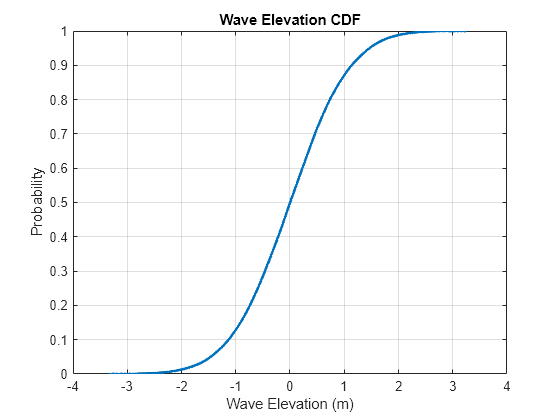
Next, estimate the significant wave height using helperEstimateSignificantWaveHeight. The estimate is obtained by taking the mean of the highest 1/3 of the wave heights, where the wave height is defined from trough-to-crest as is visually represented in the figure.
% Significant wave height
actSigHgt = helperEstimateSignificantWaveHeight(x,y,z)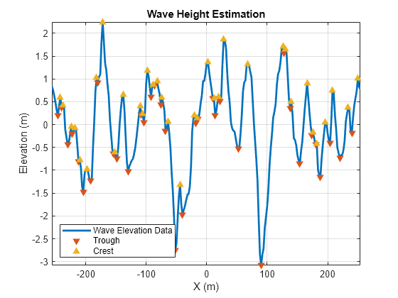
actSigHgt =
1.6340
The expected wave heights for a sea state 4 is in the range between 1.25 and 2.5 meters. Note that the simulated sea surface is within the range of expected values.
expectedSigHgt = [1.25 2.5]; % Sea state 4
actSigHgt >= expectedSigHgt(1) && actSigHgt <= expectedSigHgt(2)
ans = logical
1
Lastly, plot a subset of the sea surface heights over time to visualize the motion due to the Elfouhaily sea spectrum. Note that the simulation time for the radar data collection only runs for 2 seconds, but plot over a time period of 10 seconds to get a better sense of the motion. Uncomment helperSeaSurfaceMotionPlot to plot the moving sea surface.
% Plot sea surface motion
plotTime = 0:0.5:10; % Plot time (sec)
% helperSeaSurfaceMotionPlot(x,y,seaSurf,plotTime); % Uncomment to plot motion
Configure the Radar Transceiver
In this section, configure the radar system properties. Define the antenna and the transmitted linear frequency modulated (LFM) waveform. Assign the radar sensor to the radar platform.
% Create a radar platform using the trajectory information
rdrplat = platform(scene,'Position',rdrpos);

% Create a radar sensor looking to the East
rdr = radarTransceiver('MountingAngles',[0 depang 0],'NumRepetitions',1);

% Configure the LFM signal of the radar
rdr.Waveform = phased.LinearFMWaveform('SampleRate',fs,'PulseWidth',tpd, ...
    'PRF',prf,'SweepBandwidth',bw);

% Set receiver sample rate and noise figure
rdr.Receiver.SampleRate = fs;
rdr.Receiver.NoiseFigure = 10;

% Define transmit and receive antenna and corresponding parameters
ant = phased.SincAntennaElement('Beamwidth',azBw);
rdr.TransmitAntenna.OperatingFrequency = freq;
rdr.ReceiveAntenna.OperatingFrequency = freq;
rdr.Transmitter.Gain = antGain;
rdr.Receiver.Gain = antGain;
rdr.TransmitAntenna.Sensor = ant;
rdr.ReceiveAntenna.Sensor = ant;

% Add radar to radar platform
rdrplat.Sensors = rdr;
Generate the Datacube
Now that the scene and the radar system have been defined, generate returns from the sea surface with the clutterGenerator method and collect the IQ data using the receive method, which both reside in the radarScenario object. By default, clutterGenerator simulates clutter returns in the mainlobe. For more information about clutter modeling, see Introduction to Radar Scenario Clutter Simulation.
Use the helpers helperPlotRawIQ and helperUpdatePlotRawIQ to plot the unprocessed, raw IQ data.
% Collect clutter returns with the clutterGenerator
clutterGenerator(scene,rdr);

% Run the scenario
numSamples = 1/prf*fs;
maxRange = 20e3;
Trng = (0:1/fs:(numSamples-1)/fs);
rngGrid = [0 time2range(Trng(2:end),c)];
[~,idxTruncate] = min(abs(rngGrid - maxRange));
iqsig = zeros(idxTruncate,numPulses);
ii = 1;
hRaw = helperPlotRawIQ(iqsig);
while advance(scene)
    tmp = receive(scene); % nsamp x 1
    iqsig(:,ii) = tmp{1}(1:idxTruncate);
    if mod(ii,128) == 0
        helperUpdatePlotRawIQ(hRaw,iqsig);
    end
    ii = ii + 1;
end
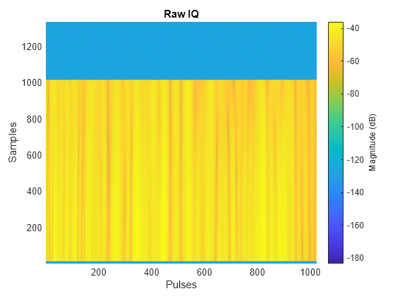
helperUpdatePlotRawIQ(hRaw,iqsig);
Process Sea Surface Returns
Use phased.RangeResponse to pulse compress the returned IQ data. Visualize the range-time behavior using helperRangeTimePlot. If the sea surface was static, you would see straight, horizontal lines in the plot, but the sea returns exhibit dynamism. At a given range, the magnitude changes with time. Note that the returns occur in a small subset of range due to the geometry (radar height, beamwidth, and depression angle).
% Pulse compress
matchingCoeff = getMatchedFilter(rdr.Waveform);
rngresp = phased.RangeResponse('RangeMethod', 'Matched filter', ...
    'PropagationSpeed',c,'SampleRate',fs);
[pcResp,rngGrid] = rngresp(iqsig,matchingCoeff);

% Plot
pcsigMagdB = mag2db(abs(pcResp));
[maxVal,maxIdx] = max(pcsigMagdB(:));
pcsigMagdB = pcsigMagdB - maxVal;
helperRangeTimePlot(rngGrid,prf,pcsigMagdB);

Use the range index of the maximum value and visualize the magnitude versus time at this range bin using helperMagTimePlot.
% Plot magnitude versus time
[idxRange,~] = ind2sub(size(pcsigMagdB),maxIdx);
helperMagTimePlot(pcsigMagdB(idxRange,:),numPulses,prf,rngGrid(idxRange));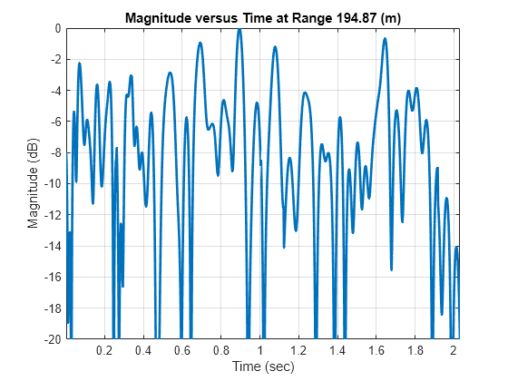
Next, generate a time-frequency plot of that same range bin using helperSTFTPlot. Generate the plot using the short-time Fourier transform function stft.
% STFT
[S,F,T] = stft(pcResp(idxRange,:),scenarioUpdateRate);
helperSTFTPlot(S,F,T,lambda,rngGrid(idxRange));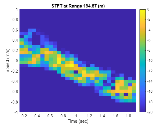
Notice that the detected speed of the range bin changes over time due to the motion of the sea surface. Over longer simulation times, periodicities are detectable.
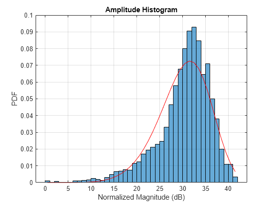
Lastly, form a histogram from the magnitude values of the data in the ranges between 180 and 210 meters using helperHistPlot. Note the shape of the histogram resembles a Weibull distribution. If you have the Statistics and Machine Learning Toolbox™, you can use the fitdist function to get the parameters for the Weibull distribution from the magnitude of the data.
% Look at a subset of data in range and convert to decibel scale
[~,idxMin] = min(abs(rngGrid - 180));
[~,idxMax] = min(abs(rngGrid - 210));
pcsigMagdB = mag2db(abs(pcResp(idxMin:idxMax,:)));

% Remove any inf values
pcsigMagdB(isinf(pcsigMagdB(:))) = [];

% Shift values to be positive
pcsigMagdB = pcsigMagdB(:) - min(pcsigMagdB(:)) + eps;

% Weibull parameters
% Note: These values can be obtained if you use fitdist(pcsigMagdB,'weibull')
scale = 32.5013;
shape = 6.3313;

% Plot histogram with theoretical PDF overlay
helperHistPlot(pcsigMagdB,scale,shape);
Summary
In this example, you learned how to:
Build a radar scenario,
Model a moving sea surface,
Investigate sea surface statistics and behavior,
Generate IQ, and
Perform time-frequency processing on simulated IQ returns.
This example can easily be extended to include targets to support applications ranging such as maritime surveillance and radar imaging.
References
Apel, John R. Principles of Ocean Physics. International Geophysics Series, v. 38. London; Orlando: Academic Press, 1987.
Elfouhaily, T., B. Chapron, K. Katsaros, and D. Vandemark. "A Unified Directional Spectrum for Long and Short Wind-Driven Waves." Journal of Geophysical Research: Oceans 102, no. C7 (July 15, 1997): 15781-96. https://doi.org/10.1029/97JC00467.
Doerry, Armin W. "Ship Dynamics for Maritime ISAR Imaging." Sandia Report. Albuquerque, New Mexico: Sandia National Laboratories, February 2008.
Ward, Keith D., Simon Watts, and Robert J. A. Tough. Sea Clutter: Scattering, the K-Distribution and Radar Performance. IET Radar, Sonar, Navigation and Avionics Series 20. London: Institution of Engineering and Technology, 2006.
Supporting Functions
helperSeaColorMap
function cmap = helperSeaColorMap(n)
% Color map for sea elevation plot

c = hsv2rgb([2/3 1 0.2; 2/3 1 1; 0.5 1 1]);
cmap = zeros(n,3);
cmap(:,1) = interp1(1:3,c(:,1),linspace(1,3,n));
cmap(:,2) = interp1(1:3,c(:,2),linspace(1,3,n));
cmap(:,3) = interp1(1:3,c(:,3),linspace(1,3,n));
end
helperSeaSurfacePlot
function helperSeaSurfacePlot(x,y,z,rdrpos)
% Plot sea elevations

% Color map for sea elevation plot
seaColorMap = helperSeaColorMap(256);

% Plot
figure
z = reshape(z,numel(x),numel(y));
surf(x,y,z)
hold on
plot3(rdrpos(1),rdrpos(2),rdrpos(3),'ok','LineWidth',2,'MarkerFaceColor','k')
legend('Sea Surface','Radar','Location','Best')
shading interp
axis equal
xlabel('X (m)')
ylabel('Y (m)')
zlabel('Elevations (m)')
stdZ = std(z(:));
minC = -4*stdZ;
maxC = 4*stdZ;
minZ = min(minC,rdrpos(3));
maxZ = max(maxC,rdrpos(3));
title('Sea Surface Elevations')
axis tight
zlim([minZ maxZ])
hC = colorbar('southoutside');
colormap(seaColorMap)
hC.Label.String = 'Elevations (m)';
hC.Limits = [minC maxC];
drawnow
pause(0.25)
end
helperSeaSurfaceCDF
function helperSeaSurfaceCDF(x)
% Calculate and plot CDF

% Form CDF
x = x(~isnan(x));
n = length(x);
x = sort(x(:));
yy = (1:n)' / n;
notdup = ([diff(x(:)); 1] > 0);
xx = x(notdup);
yy = [0; yy(notdup)];

% Create vectors for plotting
k = length(xx);
n = reshape(repmat(1:k, 2, 1),2*k,1);
xCDF = [-Inf; xx(n); Inf];
yCDF = [0; 0; yy(1+n)];

% Plot
figure
plot(xCDF,yCDF,'LineWidth',2)
grid on
title('Wave Elevation CDF')
xlabel('Wave Elevation (m)')
ylabel('Probability')
drawnow
pause(0.25)
end
helperEstimateSignificantWaveHeight
function sigHgt = helperEstimateSignificantWaveHeight(x,y,z)
% Plot an example showing how the wave heights are estimated and estimate
% the significant wave height

% Plot wave height estimation
figure
numX = numel(x);
z = reshape(z,numX,numel(y));
zEst = z(numX/2 + 1,:);
plot(x,zEst,'LineWidth',2)
grid on
hold on
xlabel('X (m)')
ylabel('Elevation (m)')
title('Wave Height Estimation')
axis tight
idxMin = islocalmin(z(numel(x)/2 + 1,:));
idxMax = islocalmax(z(numel(x)/2 + 1,:));
co = colororder;
plot(x(idxMin),zEst(idxMin),'v', ...
    'MarkerFaceColor',co(2,:),'MarkerEdgeColor',co(2,:))
plot(x(idxMax),zEst(idxMax),'^', ...
    'MarkerFaceColor',co(3,:),'MarkerEdgeColor',co(3,:))
legend('Wave Elevation Data','Trough','Crest','Location','SouthWest')

% Estimate significant wave height
waveHgts = [];
for ii = 1:numX
    zEst = z(ii,:);
    idxMin = islocalmin(zEst);
    troughs = zEst(idxMin);
    numTroughs = sum(double(idxMin));
    idxMax = islocalmax(zEst);
    crests = zEst(idxMax);
    numCrests = sum(double(idxMax));
    numWaves = min(numTroughs,numCrests);
    waveHgts = [waveHgts ...
        abs(crests(1:numWaves) - troughs(1:numWaves))]; %#ok<AGROW>
end
waveHgts = sort(waveHgts);
idxTopThird = floor(numel(waveHgts)*2/3);
sigHgt = mean(waveHgts(idxTopThird:end));
drawnow
pause(0.25)
end
helperSeaSurfaceMotionPlot
function helperSeaSurfaceMotionPlot(x,y,seaSurf,plotTime) %#ok<DEFNU>
% Color map for sea elevation plot
seaColorMap = helperSeaColorMap(256);

% Get initial height
[xGrid,yGrid] = meshgrid(x,y);
z = height(seaSurf,[xGrid(:).'; yGrid(:).'],plotTime(1));

% Plot
hFig = figure;
hS = surf(x,y,reshape(z,numel(x),numel(y)));
hold on
shading interp
axis equal
xlabel('X (m)')
ylabel('Y (m)')
zlabel('Elevations (m)')
stdZ = std(z(:));
minZ = -4*stdZ;
maxZ = 4*stdZ;
title('Sea Surface Motion Plot')
xlim([-50 50])
ylim([-50 50])
zlim([minZ maxZ])
hC = colorbar('southoutside');
colormap(seaColorMap)
hC.Label.String = 'Elevations (m)';
hC.Limits = [minZ maxZ];
view([-45 12])

% Change figure size
ppos0 = get(hFig,'Position');
figWidth = 700;
figHeight = 300;
set(gcf,'position',[ppos0(1),ppos0(2),figWidth,figHeight])

numTimes = numel(plotTime);
for ii = 2:numTimes
    % Update plot
    z = height(seaSurf,[xGrid(:).'; yGrid(:).'],plotTime(ii));
    hS.ZData = reshape(z,numel(x),numel(y));
    drawnow
    pause(0.1)
end
pause(0.25)
end
helperPlotRawIQ
function hRaw = helperPlotRawIQ(iqsig)
% Plot raw IQ magnitude

figure()
hRaw = pcolor(mag2db(abs(iqsig)));
hRaw.EdgeColor = 'none';
title('Raw IQ')
xlabel('Pulses')
ylabel('Samples')
hC = colorbar;
hC.Label.String = 'Magnitude (dB)';
drawnow
pause(0.25)
end
helperUpdatePlotRawIQ
function helperUpdatePlotRawIQ(hRaw,iqsig)
% Update the raw IQ magnitude plot

hRaw.CData = mag2db(abs(iqsig));
drawnow
pause(0.25)
end
helperRangeTimePlot
function helperRangeTimePlot(rngGrid,prf,pcsigMagdB)
% Range-Time Plot

figure()
numPulses = size(pcsigMagdB,2);
hImage = pcolor((1:numPulses)*1/prf,rngGrid,pcsigMagdB);
hImage.EdgeColor = 'none';
shading interp
xlabel('Time (sec)')
ylabel('Range (m)')
hC = colorbar;
hC.Label.String = 'Magnitude (dB)';
axis tight
title('Range versus Time')
clim([-20 0])
ylim([140 260])
drawnow
pause(0.25)
end
helperMagTimePlot
function helperMagTimePlot(magVals,numPulses,prf,rngVal)
% Magnitude vs. Time Plot

figure()
plot((1:numPulses)*1/prf,magVals,'LineWidth',2)
grid on
xlabel('Time (sec)')
ylabel('Magnitude (dB)')
axis tight
title(sprintf('Magnitude versus Time at Range %.2f (m)',rngVal))
ylim([-20 0])
drawnow
pause(0.25)
end
helperSTFTPlot
function helperSTFTPlot(S,F,T,lambda,rngVal)
% Time-Frequency Plot

figure()
S = mag2db(abs(S)); % Convert to dB
S = S - max(S(:)); % Normalize
Speed = dop2speed(F,lambda)/2; % Speed (m/s)
hSTFT = pcolor(T,Speed,S);
hold on
hSTFT.EdgeColor = 'none';
colorbar
xlabel('Time (sec)')
ylabel('Speed (m/s)')
title(sprintf('STFT at Range %.2f (m)',rngVal))
clim([-20 0])
ylim([-1 1])
drawnow
pause(0.25)
end
helperHistPlot
function helperHistPlot(pcsigMagdB,scale,shape)
% Amplitude Distribution

% Histogram
figure
hHist = histogram(pcsigMagdB,'Normalization','pdf'); % Create histogram
grid on
hold on
xlabel('Normalized Magnitude (dB)')
ylabel('PDF')
title('Amplitude Histogram')

% Lognormal overlay
edges = hHist.BinEdges;
x = (edges(2:end) + edges(1:end-1))./2;
z = x./scale;
w = exp(-(z.^shape));
y = z.^(shape - 1).*w .*shape./scale;
plot(x,y,'-r')
end